Global Financial Cycle Transmission to Indonesian Commercial Bank Balance Sheets: Bank-Level Panel Evidence, 2002–2025
*HAMPARAN Institute (PT Hamparan Berkah Teknologi), Jember, Indonesia. ORCID: 0000-0003-0209-834X. Email: [email protected]. The author thanks the Otoritas Jasa Keuangan (OJK) for the public Commercial Bank Quarterly Financial Reports database used in this paper. All errors are the author's own.
Abstract
This paper estimates the bank-level transmission of the global financial cycle to Indonesian commercial banks (BUK) over 2002–2025. A composite cycle factor is the first principal component of five US financial-market series; bank-level local projections are estimated at horizons of one to five years. A one-standard-deviation shock raises three-year credit growth by 4.6 log points (\(p < 0.01\)), lowers NPL by 25 basis points, and compresses CAR by 80 basis points. Post-2016 sensitivity is roughly four times pre-2014 magnitude, while the 2022–23 Fed-hike episode produces credit expansion alongside falling NPL — evidence of asymmetric macroprudential effectiveness containing downside but not upside transmission.
JEL classification: G21 (Banks; Depository Institutions), F32 (Current Account Adjustment; Short-Term Capital Movements), E58 (Central Banks and Their Policies), G28 (Government Policy and Regulation).
Keywords: global financial cycle; bank balance sheets; Indonesia; macroprudential policy; local projections; capital flow transmission.
1. Introduction
The proposition that a single global financial cycle drives capital flows, credit growth, and asset prices across emerging-market economies — articulated by Rey (2013, 2016) and formalised by Miranda-Agrippino and Rey (2020, 2022) — has become a benchmark for international macro-finance. The transmission operates through cross-border banking flows (Bruno and Shin 2015a, 2015b) and the dollar funding channel (Avdjiev, McCauley, and Shin 2016), and its asymmetric interaction with macroprudential policy is documented across 119 countries by Cerutti, Claessens, and Laeven (2017) and across 57 economies by Akinci and Olmstead-Rumsey (2018). The IMF’s October 2025 Global Financial Stability Report and World Economic Outlook (IMF 2025a, 2025b) flag the cycle as a continuing first-order driver of emerging-market financial stability.
Indonesia is an unusually informative laboratory for these questions. Its banking system is the largest in ASEAN by assets, the capital account is open, and Bank Indonesia’s deputy-governor Warjiyo (2016) describes the domestic policy architecture as a “policy mix” of inflation targeting, exchange-rate management, capital-flow management, and macroprudential instruments deployed in three waves: loan-to-value ratios from 2012, the countercyclical capital buffer regulation from 2015, and foreign-currency hedging rules for non-bank corporates from 2014. The Financial System Crisis Prevention and Resolution Law (PPKSK, 2016) formalised inter-agency coordination through the Komite Stabilitas Sistem Keuangan. The most recent IMF Article IV consultation and Financial Sector Assessment Program (IMF 2024a, 2024b) judge the framework as highly resilient through the 2020 COVID shock and the 2022–23 Fed hike cycle, providing a sharp pre/post identification window centred on the 2016 reform.
Bank-level Indonesian evidence on global cycle transmission remains scarce. Existing studies operate primarily at the aggregate cross-country level (Cerutti, Claessens, and Ratnovski 2017; Forbes and Warnock 2012) or focus on a single shock window (Basri 2017 on the 2013 Taper; Soedarmono, Gunadi, Indawan, and Wulandari 2022 through the 2022 Fed liftoff). The single-country Indonesian bank-level work that does exist — Catalán, Hoffmaister, and Harun (2020) on the nonlinear bank capital–lending response and Soedarmono, Gunadi, Pambudi, and Nurhayati (2021) on the domestic bank-lending channel — is designed to identify domestic monetary transmission rather than global cycle propagation. None of these designs can identify the cross-sectional heterogeneity — by ownership, size, or foreign-currency exposure — through which the global cycle actually reaches Indonesian banks.
This paper closes that gap on four margins. First, it constructs a public-data bank-level panel of all 97 commercial banks (Bank Umum Konvensional, BUK) spanning 2002–2025, combining a continuous outcome panel of assets, credit, and deposits with a bridged capital-adequacy and asset-quality panel, a foreign-currency exposure proxy built from off-balance-sheet commitments, and a composite global financial cycle factor estimated by principal-component analysis on five US financial-market series. Second, it estimates local projections (Jordà 2005; Plagborg-Møller and Wolf 2021; Jordà and Taylor 2023) of cumulative credit, asset, NPL, and CAR responses to the cycle factor at horizons of one to five years. Third, it documents heterogeneity by bank ownership type, size quintile, and FX-exposure quartile, and recovers the bank-level response to six pre-specified risk-off episodes. Fourth, it provides the first single-country bank-level evidence of asymmetric macroprudential effectiveness in Indonesia — a pattern previously visible only in cross-country panels.
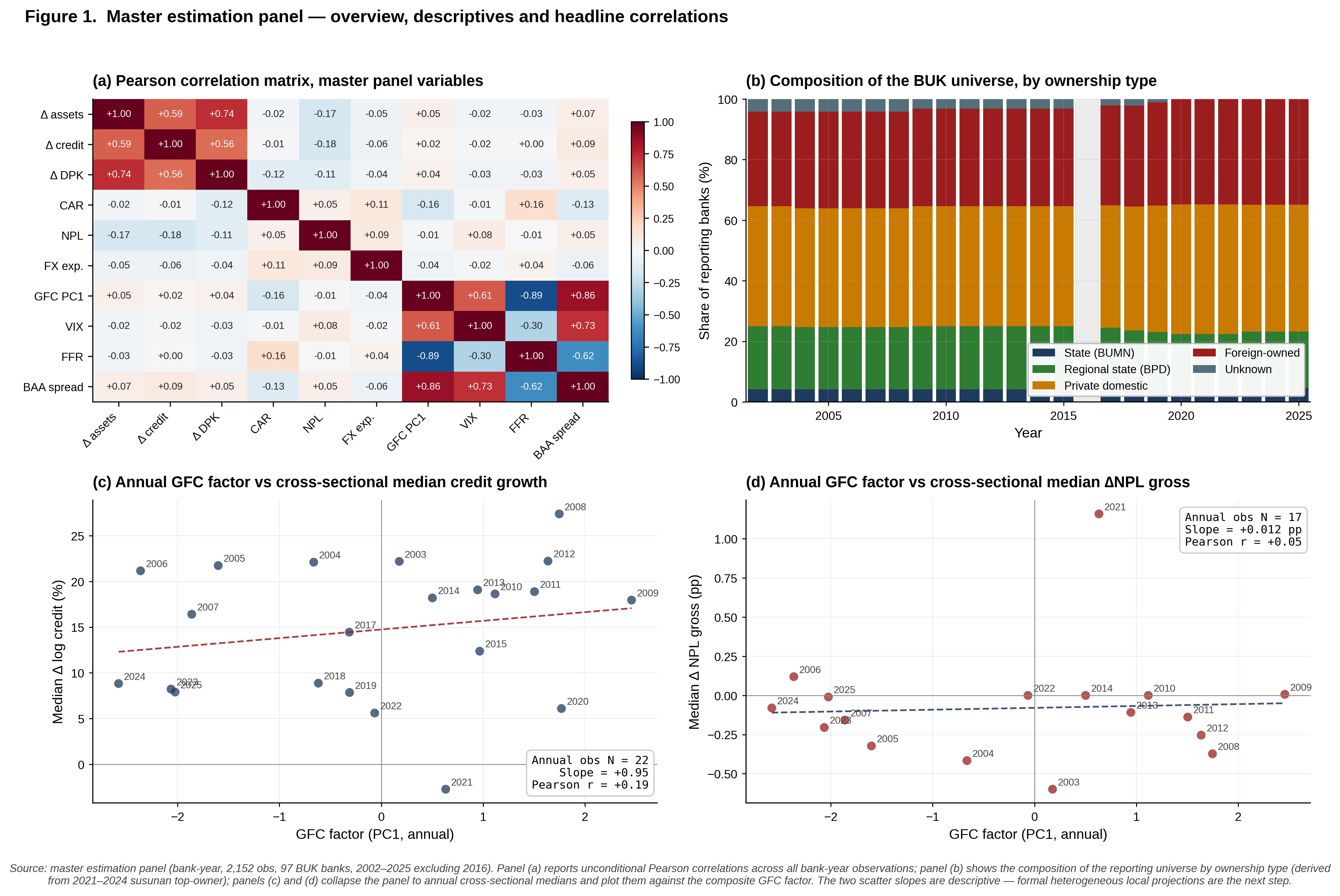
Three findings stand out. The unconditional annual correlation between the global cycle factor and the median bank-level credit growth is weak (+0.19), suggesting at first glance that Indonesian banking is unresponsive — yet bank-level local projections recover a precisely estimated +4.6 log-point cumulative credit response at the three-year horizon (p < 0.01), with NPL falling 25 basis points and CAR compressing 80 basis points. Ownership type, not bank size, dominates the heterogeneous response: state banks exhibit a recapitalisation signature under stress (NPL up, CAR also up) while high-FX-exposure banks deleverage materially. The post-2016 sensitivity of credit growth to the global cycle is roughly four times the pre-2014 magnitude, and the 2022–23 Fed-hike episode delivers stable credit and declining NPL — sharply different from the GFC 2008–09 and COVID-19 patterns. Together the evidence describes a macroprudential framework that contains downside transmission but does not contain the upside; the cross-country asymmetry of Cerutti et al. (2017), Akinci and Olmstead-Rumsey (2018), Fendoglu (2017), and Frost, Ito, and van Stralen (2020) holds within a single jurisdiction.
The remainder proceeds as follows. Section 2 reviews the related literature in five strands. Section 3 describes the data. Section 4 lays out the empirical strategy. Section 5 reports the baseline local projections. Section 6 examines heterogeneity. Section 7 presents the episode event-study. Section 8 reports robustness. Section 9 interprets the asymmetric-macroprudential narrative. Section 10 discusses policy implications. Section 11 concludes.
2. Related literature
This paper sits at the intersection of five strands of work, briefly reviewed below.
2.1 The global financial cycle and its measurement
The empirical regularity that US “push” factors drive emerging-market capital flows, asset prices, and credit conditions dates at least to Calvo, Leiderman, and Reinhart (1993). Rey (2013) sharpened the proposition into the “dilemma not trilemma”: flexible exchange rates and capital mobility are not sufficient to insulate periphery countries from the global cycle. Miranda-Agrippino and Rey (2020) operationalised the cycle as the first principal component of a global asset-price panel, attributing roughly twenty per cent of cross-asset variance to this factor and identifying US monetary policy shocks as a leading driver; their Handbook treatment (Miranda-Agrippino and Rey 2022) extends the framework to the dollar funding channel. Borio and Disyatat (2011), updated by Aldasoro, Avdjiev, Borio, and Disyatat (2023), offer the complementary “excess elasticity” view, in which the international monetary system’s accommodation of global credit creation — not US monetary policy per se — does the heavy lifting; the two narratives agree on the empirical regularity of cross-border transmission but differ on policy implications. The composite global financial cycle factor constructed in this paper follows the Miranda-Agrippino–Rey principal-component approach and augments their five-series panel with the BAA — 10-year corporate-credit spread, which Gilchrist and Zakrajšek (2012) identify as a parsimonious summary of US financial conditions.
2.2 Bank-level transmission of global liquidity
Bruno and Shin (2015a) develop a “double-decker” model of cross-border banking in which regional banks borrow dollars from global banks to fund local-currency lending — leverage at the global-bank tier amplifies the international transmission. Bruno and Shin (2015b) document the empirical risk-taking channel: when the VIX is low and dollar funding is cheap, cross-border bank leverage rises and capital flows to EMs accelerate. Avdjiev, McCauley, and Shin (2016) formalise the dollar’s role as the unit of account in cross-border bank credit and show that the dollar exchange rate is itself a key transmission variable — a stronger dollar tightens financial conditions in EM banking systems independently of the path of US interest rates.
Bank-level evidence has accumulated more slowly. Cerutti, Claessens, and Ratnovski (2017) confirm the aggregate cycle using BIS cross-border bank credit data but cannot resolve bank-level heterogeneity; Bräuning and Ivashina (2020) use syndicated-loan data to document sharp rebalancing of emerging-market exposures by global banks during US monetary tightening; and Arnabal, Camara, and Dassatti (2025), using Uruguayan credit-registry data to identify high-frequency shocks to global banks’ net worth, find that better-capitalised local banks transmit global credit easing more strongly. No comparable single-country bank-level panel exists for Indonesia.
2.3 Macroprudential policy effectiveness
Cerutti, Claessens, and Laeven (2017) reshaped this literature with a 119-country panel of macroprudential instrument use over 2000–2013. Their headline finding is that macroprudential tightening generally slows credit growth, but with three asymmetries: (a) effects are weaker in advanced economies, (b) effects are weaker in busts than in booms, and (c) tools targeting borrowers (loan-to-value, debt-to-income) are more effective than tools targeting lenders (capital buffers). Akinci and Olmstead-Rumsey (2018) sharpen the borrower-versus-lender distinction and confirm the upside-versus-downside asymmetry using a panel of 57 economies.
For emerging markets specifically, Fendoglu (2017) finds that borrower-based tools, measures with a domestic focus, and domestic reserve requirements are particularly effective at containing credit cycles. More recent evidence from Frost, Ito, and van Stralen (2020) and Epure, Mihai, Minoiu, and Peydró (2024) sharpens the picture: when the VIX is low, tighter macroprudential policies reduce household lending — particularly riskier foreign-currency and high debt-service-to-income loans, and lending by banks dependent on foreign funding — while less-regulated local-currency lending to real-estate firms expands. Macroprudential tools shift, rather than eliminate, the channel through which the global cycle transmits to local credit — a pattern directly relevant to the Indonesian results that follow.
2.4 Indonesia-specific evidence
Bank Indonesia’s policy mix is authoritatively described in Warjiyo (2016) and Warjiyo and Juhro (2019). The framework rests on five pillars: (i) interest-rate policy under inflation targeting; (ii) exchange-rate management with the “balanced” approach; (iii) capital-flow management; (iv) macroprudential instruments (LTV ratios from 2012, loan-to-funding-linked reserve requirements, the countercyclical capital buffer from 2015, and FX hedging rules for corporates from 2014); and (v) crisis-management coordination through the Komite Stabilitas Sistem Keuangan established under Law No. 9 of 2016 (PPKSK). Warjiyo (2016) reports that 92 per cent of the 2,400 corporates required to comply with the 2014 FX hedging rule were in compliance by 2016. Dąbrowski and Widiantoro (2023), using a structural VAR over 2003–2020, conclude that LTV tightening is effective at containing housing-credit growth in the medium run, while real property-price responses display the price-puzzle pattern familiar from monetary-policy VARs.
On the bank balance-sheet response, Catalán, Hoffmaister, and Harun (2020) document a nonlinear capital–lending relationship in a panel of Indonesian banks 2001Q1–2018Q4: weakly capitalised banks respond more strongly to capital changes than well-capitalised banks — a finding that motivates the separate analysis of the CAR margin reported in Section 5. Soedarmono, Gunadi, Pambudi, and Nurhayati (2021) study the domestic bank-lending channel and find that it operates with a roughly two-quarter lag and is conditional on the absence of credit-crunch conditions, supporting the bank-capital channel.
On capital flows specifically, Basri (2017) documents Indonesia’s response to the 2013 Taper tantrum and concludes that the policy mix of monetary tightening, flexible exchange-rate management, and contractionary fiscal policy enabled the country to exit the “Fragile Five” within seven months. Soedarmono, Gunadi, Indawan, and Wulandari (2022) update Basri’s analysis through the 2022 Fed-hike episode and find that higher foreign capital inflows mitigate aggregate bank credit risk in Indonesia. None of these studies builds the 24-year bank-level panel of all 97 commercial banks assembled here, and none separates the upside from the downside transmission of the global cycle.
2.5 Local projections in panel settings
The local-projection framework of Jordà (2005) has become the workhorse for impulse-response estimation in panel data, and Plagborg-Møller and Wolf (2021) show that local projections and VAR estimators are asymptotically equivalent in many settings. Two recent contributions sharpen inference for the panel case. Montiel-Olea and Plagborg-Møller (2021) prove that lag-augmented local projections support standard inference with normal critical values uniformly over stationary and persistent regressors, and obviate the need to correct standard errors for serial correlation. Almuzara and Sancibrián (2024) extend the panel case explicitly: when aggregate shocks drive the variation of interest, including lags as controls and clustering standard errors at the time level yields valid inference regardless of the signal-to-noise ratio of the shock. The panel used here has 97 banks and 23 effective time periods; the cross-sectional dimension dominates the time dimension, so bank-clustered standard errors are the primary inference choice, with two-way clustering on bank and year reported as a robustness check (Section 8). Jordà and Taylor’s (2023) review of “Local Projections for Applied Economics” provides best-practice guidance on horizon selection, lag-augmentation, and the handling of fixed effects, all of which are followed below.
3. Data
3.1 Overview
This paper assembles an annual bank-year panel of all 97 commercial banks (Bank Umum Konvensional, BUK) authorised by the Otoritas Jasa Keuangan (OJK) over 2002–2025, excluding the structural reporting gap in fiscal year 2016. Three primary sources are used: bank balance-sheet, risk, and ownership variables from the OJK Commercial Bank Financial Reports (CFS) archive; the composite global financial cycle factor and its six episode windows constructed from US financial-market series in the Federal Reserve Economic Data (FRED) repository; and three domestic macroeconomic controls (BI policy rate, IDR–USD exchange rate, Indonesia headline CPI) also from FRED. The full data scope is summarised in Table 1. The working sample for the local projections contains 2,055 bank-year observations after dropping bank-years missing the lagged log-asset control. Variable construction details — label bridging, format reconciliation, and classification rules — are documented in Appendix C.
Table 1. Data scope — variables, units, sources, sample sizes, and central tendency
| # | Variable | Description | Unit | Source | N obs | Mean | Median |
|---|---|---|---|---|---|---|---|
| 1 | Total assets | Bank balance-sheet total | IDR trillion | OJK CFS posisi_keuangan_bulanan |
2,152 | 53.8 | 11.1 |
| 2 | Total credit | Loans extended (excl. inter-bank) | IDR trillion | OJK CFS posisi_keuangan_bulanan |
2,150 | 32.4 | 5.9 |
| 3 | Third-party deposits (DPK) | Giro + tabungan + simpanan berjangka + deposito | IDR trillion | OJK CFS posisi_keuangan_bulanan |
2,150 | 39.1 | 7.5 |
| 4 | Capital adequacy ratio (CAR) | Regulatory capital / risk-weighted assets | Percent | OJK CFS kpmm_konsolidasi + rasio_keuangan (2021+) |
1,481 | 28.4 | 22.2 |
| 5 | NPL gross ratio | (Substandard + Doubtful + Loss) / Total credit | Percent | OJK CFS kualitas_aktiva_produktif + rasio_keuangan (2021+) |
1,677 | 3.7 | 2.4 |
| 6 | FX exposure ratio | Off-balance-sheet FX commitments / Total assets | Ratio | OJK CFS komitmen_kontinjensi + spot_derivatif |
2,289 | 0.25 | 0.01 |
| 7 | Bank ownership type | State / BPD / Private domestic / Foreign | Categorical (4) | OJK CFS susunan 2021–2024 |
97 banks | — | — |
| 8 | Bank size quintile | Within-year asset quintile | Ordinal 1–5 | Derived from #1 | 2,152 | 3.0 | 3.0 |
| 9 | FX exposure quartile | Within-period FX-exposure quartile | Ordinal 1–4 | Derived from #6 | 2,289 | 2.5 | 2.5 |
| 10 | GFC factor (PC1) | First principal component of 5 US financial-market series | Standard deviation | FRED: VIXCLS, DTWEXBGS, DFF, DGS10, BAA10Y | 23 annual | 0.00 | 0.14 |
| 11 | Episode dummies (×6) | GFC 2008–09, Taper 2013, CNY 2015–16, EM 2018, COVID 2020, FH 2022–23 | 0/1 | Coded from #10 + literature | 23 years | — | — |
| 12 | BI policy rate | Bank Indonesia policy rate | Percent | FRED IRSTCI01IDM156N | 23 years | 7.5 | 6.6 |
| 13 | IDR–USD depreciation | Year-on-year log change | Percent | FRED CCUSMA02IDM618N | 24 years | 2.8 | 3.8 |
| 14 | CPI inflation | Year-on-year headline | Percent | FRED IDNCPIALLMINMEI | 24 years | 5.8 | 5.3 |
Notes: Sample 2002–2025 excluding fiscal-year 2016 (structural OJK gap). Balance-sheet means/medians reported in IDR trillion (1 trillion = 10¹² IDR); regression specifications use within-bank log differences. Mean/median for variable #7 (ownership type) and #11 (episode dummies) omitted as non-numeric; ownership distribution is given in §3.5, episode windows in §3.6. Variables #8 and #9 are derived ordinal ranks (means equal mid-quantile by construction). Variable #10 is z-scored at construction. Full descriptive moments — SD, p10, p90 — are reported in Table B5.
3.2 Bank balance-sheet variables
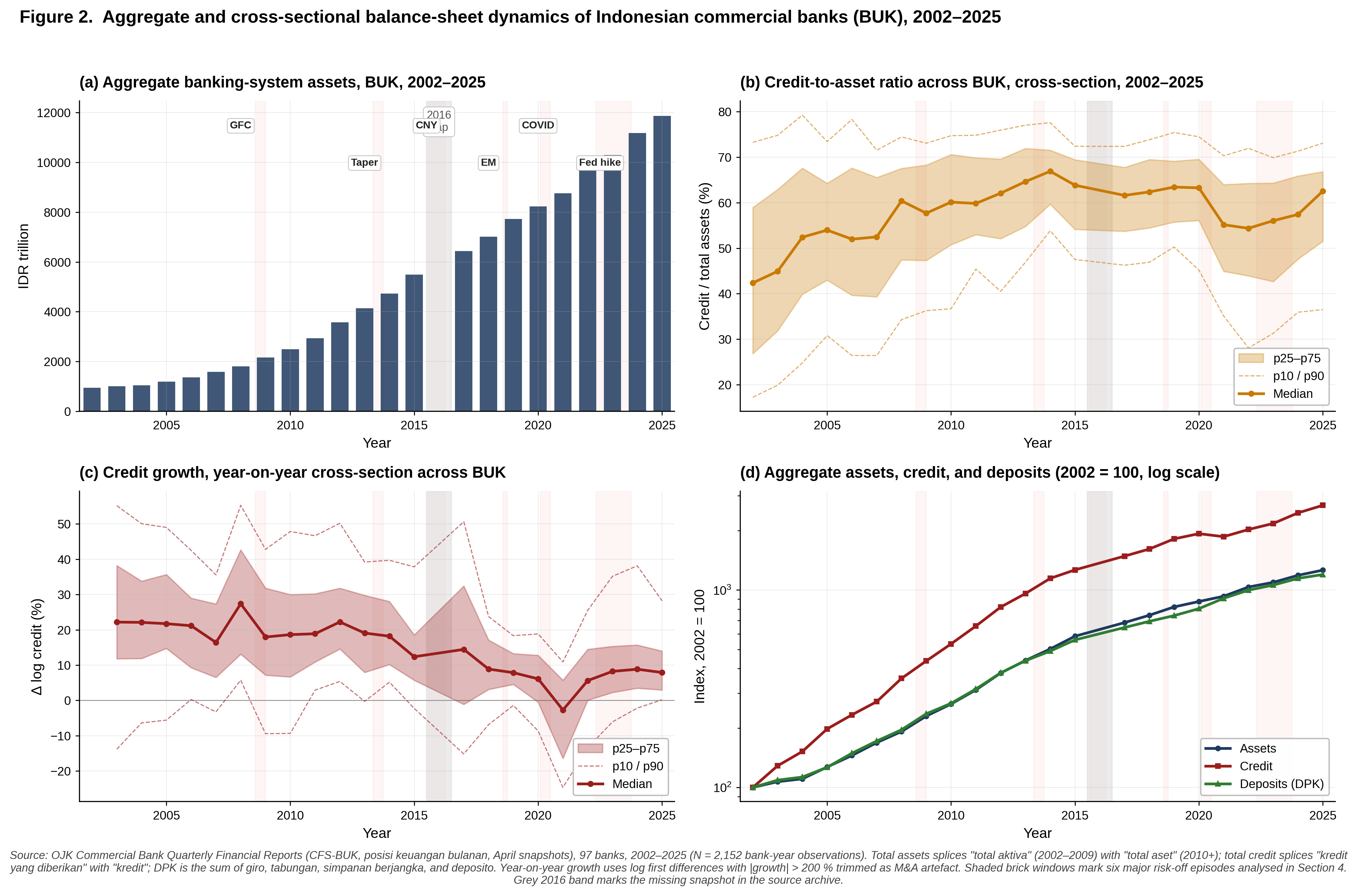
Total assets, total credit, and total third-party deposits (Dana Pihak Ketiga, DPK) are extracted from the OJK posisi keuangan reports and spliced across the pre-2010 and 2010+ label conventions (Appendix A.2). Year-on-year log growth is computed within each bank; growth above 200 per cent is set to missing as an M&A artefact.
3.3 Risk variables
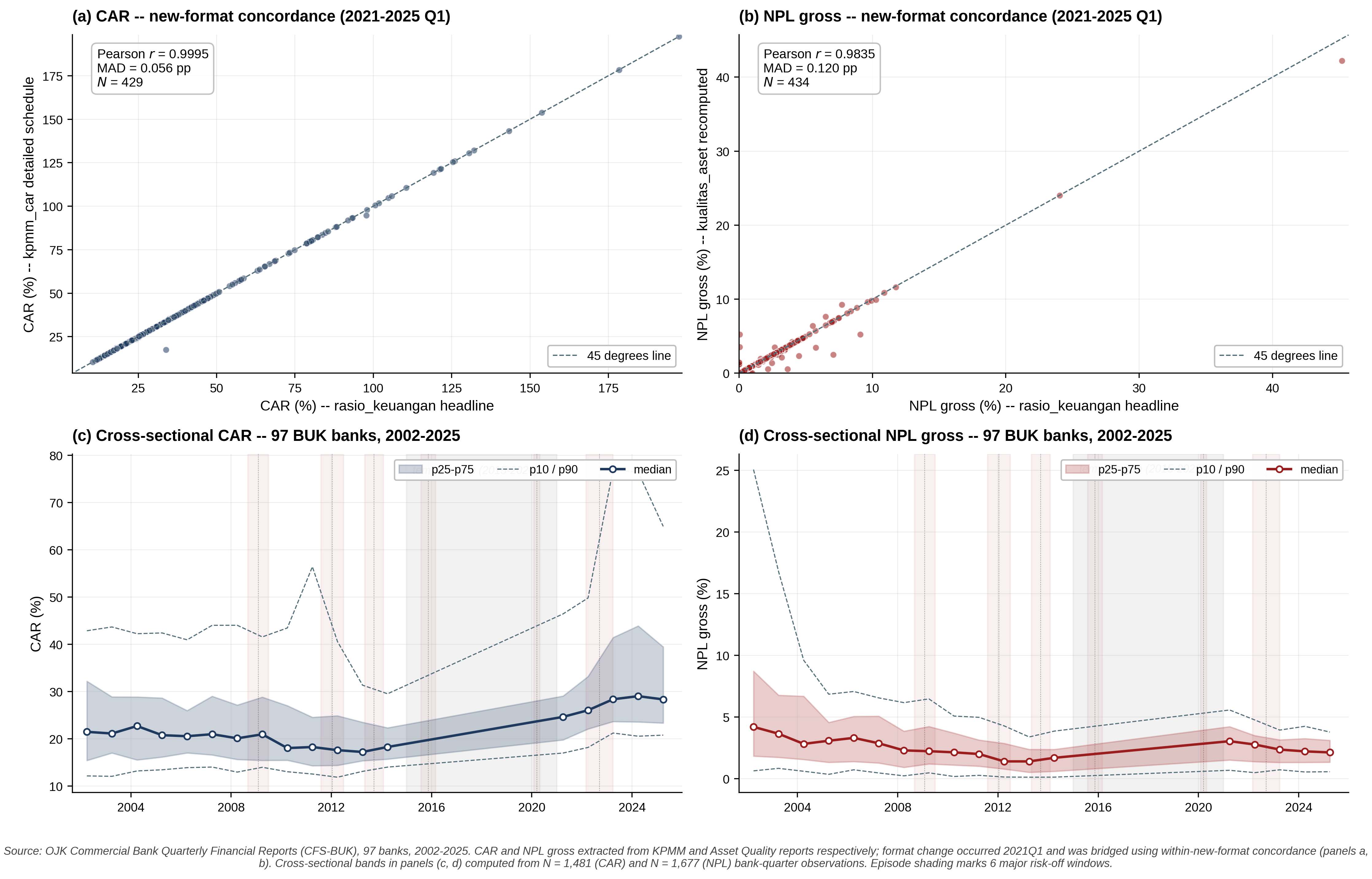
The capital adequacy ratio (CAR) and the gross non-performing loan ratio (NPL gross) measure loss-absorbing capacity and asset-quality stress respectively. Both are bridged across the pre-2021 OJK template (kpmm_konsolidasi, kualitas_aktiva_produktif) and the post-2021 rasio_keuangan, with within-format concordance Pearson r ≈ 0.99 (Appendix A.3).
3.4 Foreign-currency exposure
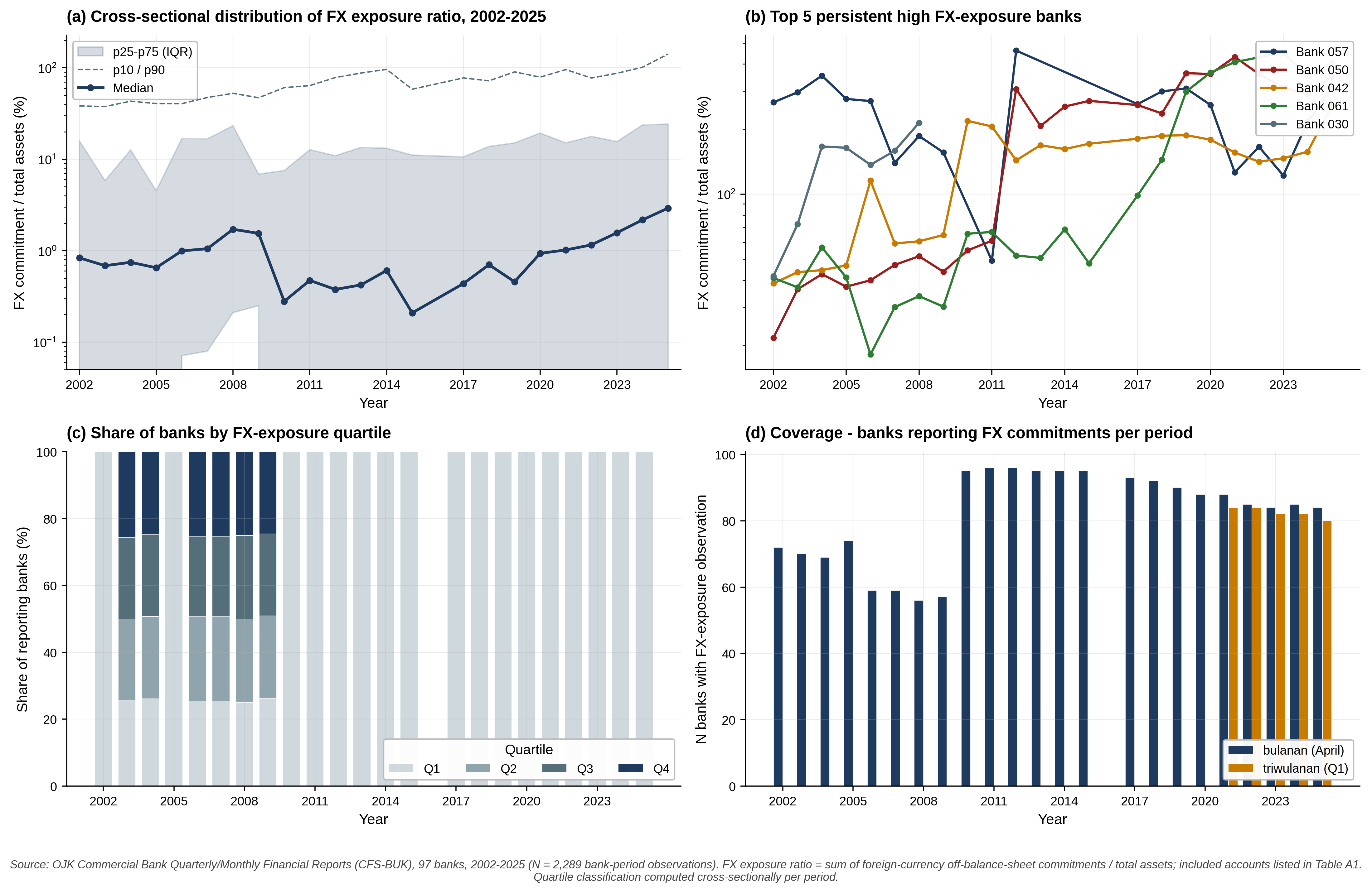
Bank-level FX exposure is proxied by the ratio of off-balance-sheet foreign-currency commitments to total assets, aggregating eleven account labels from the OJK komitmen kontinjensi and spot derivatif reports (Appendix A.4). The bulanan-to-triwulanan cross-validation yields Pearson r = 0.925.
3.5 Bank characteristics
Three bank-level characteristics enter the heterogeneity specifications: a four-class ownership type — 4 state-owned (BUMN), 20 regional state (Bank Pembangunan Daerah, BPD), 38 private domestic, and 31 foreign-owned banks, with 4 unclassified due to missing susunan coverage — derived from the 2021–2024 ownership-disclosure records; a within-year asset size quintile; and a within-period FX-exposure quartile. Classification rules are in Appendix A.5.
3.6 Global financial cycle factor
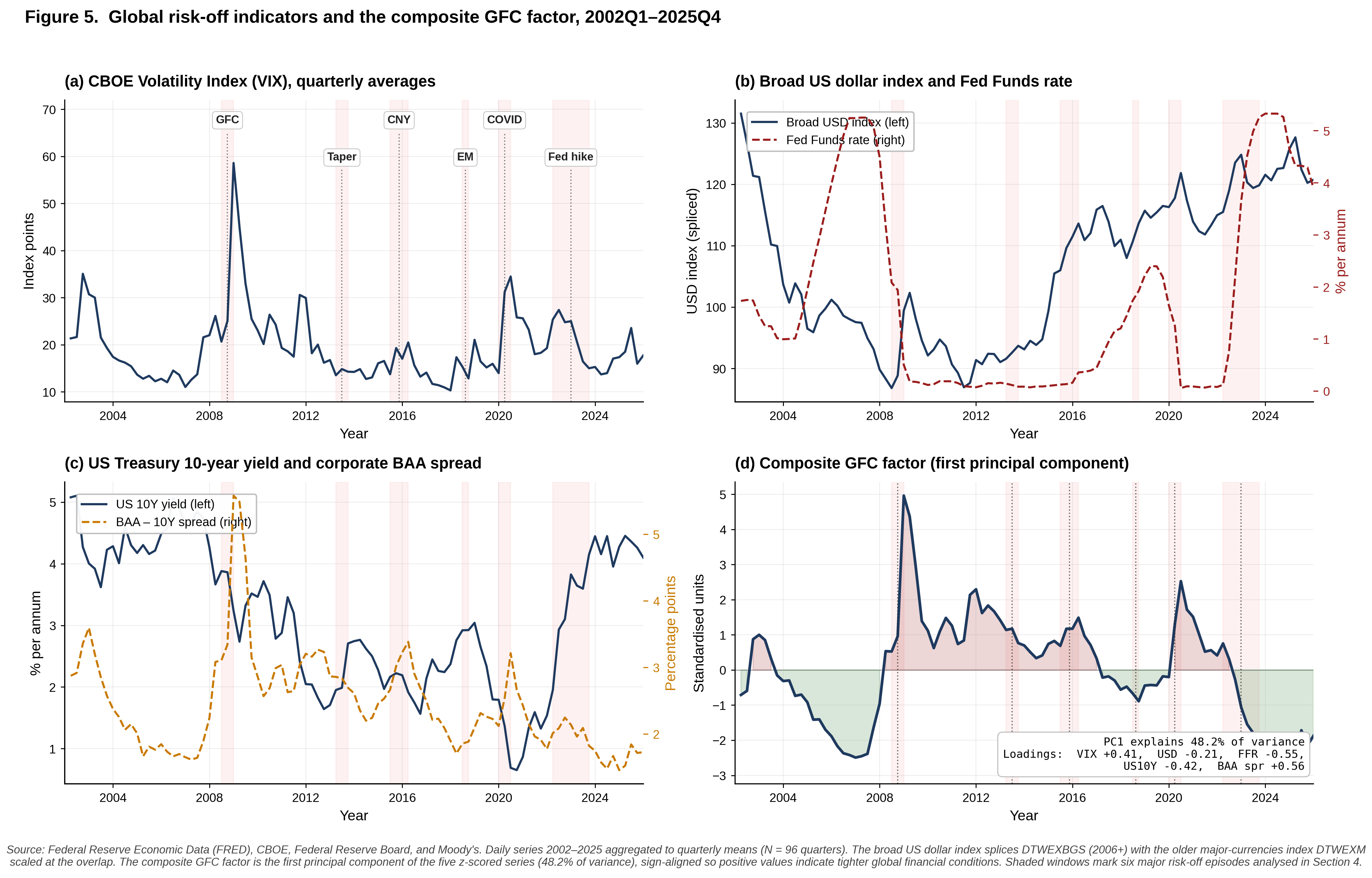
The composite global financial cycle factor is the first principal component of five z-scored US financial-market series — the VIX, the broad US dollar index, the Fed Funds rate, the 10-year Treasury yield, and the Moody’s BAA — 10-year corporate spread — aggregated to quarterly means. PC1 explains 48.2 per cent of cross-indicator variance with the sign aligned so that positive values denote risk-off conditions (Appendix A.6). Six pre-specified episode dummies code year-overlap with the major risk-off windows: the global financial crisis (2008Q3–Q4), the Federal Reserve taper tantrum (2013Q2–Q3), the Chinese renminbi devaluation and commodity bust (2015Q3–2016Q1), the emerging-market contagion (2018Q3), the COVID-19 risk-off (2020Q1–Q2), and the Federal Reserve hike cycle (2022Q2–2023Q3).
3.7 Domestic macroeconomic controls
Three domestic time-series controls enter the robustness specifications, all from FRED and aggregated to annual means: the Bank Indonesia policy rate, the IDR–USD exchange rate (year-on-year log depreciation), and the Indonesia headline CPI (year-on-year inflation).
4. Empirical strategy
4.1 Local projections framework
The baseline empirical model is a sequence of local projections (Jordà 2005) in which the cumulative h-year change in the bank-level outcome is regressed on the contemporaneous global financial cycle shock, with bank fixed effects and lagged bank-level controls:
\[ y_{i,t+h} - y_{i,t} = \alpha_i + \beta_h \, \mathrm{GFC}_t + \bm{\gamma}_h^{\prime} \, \bm{X}_{i,t-1} + \varepsilon_{i,t+h}, \tag{1} \]
where the outcomes \(y \in \{\ln \mathrm{credit},\, \ln \mathrm{assets},\, \mathrm{NPL}_{\mathrm{gross}},\, \mathrm{CAR}\}\), the horizons \(h \in \{1, 2, 3, 5\}\) years, and \(\bm{X}_{i,t-1}\) collects three lagged bank-level controls: log total assets (size), the DPK share of total liabilities (funding structure), and the credit-to-asset ratio (asset mix). Bank fixed effects \(\alpha_i\) absorb time-invariant heterogeneity in business model, ownership, and regional exposure. The coefficient of interest is \(\beta_h\), interpreted as the cumulative h-year response of the outcome to a one-standard-deviation increase in the global cycle factor. Standard errors are clustered by bank to allow within-bank serial correlation, with two-way clustering on bank and year reported as a robustness check (Section 8).
The shock variable is the Q1 reading of the GFC factor, which lines up with the April BUK reporting date and minimises within-year overlap with the dependent variable.
4.2 Heterogeneity specification
To recover heterogeneous responses, the baseline is augmented with bank-characteristic interactions and year fixed effects:
\[ y_{i,t+h} - y_{i,t} = \alpha_i + \delta_t + \sum_{k \in \mathcal{K}} \lambda_{h,k} \, \bigl(\mathrm{GFC}_t \times Z_{i,t,k}\bigr) + \bm{\gamma}_h^{\prime} \, \bm{X}_{i,t-1} + \varepsilon_{i,t+h}, \tag{2} \]
where \(\mathcal{K}\) indexes the categorical heterogeneity variables: ownership type (state, regional state, private domestic, with foreign as the omitted reference), within-year asset size quintile (with quintile 1 as the omitted reference), and within-period FX-exposure quartile (with quartile 1 as the omitted reference). Year fixed effects \(\delta_t\) absorb the main effect of the GFC factor, so the reported \(\lambda_{h,k}\) measure the additional response of each group relative to its omitted reference category.
4.3 Episode event-study
To assess whether specific risk-off windows drive the average effect, the GFC factor is replaced with each of six episode dummies in turn, retaining bank fixed effects but dropping year fixed effects (year FE would absorb the episode dummy):
\[ y_{i,t+h} - y_{i,t} = \alpha_i + \theta_{e,h} \, \mathbb{1}\{t \in e\} + \bm{\gamma}_h^{\prime} \, \bm{X}_{i,t-1} + \varepsilon_{i,t+h}, \tag{3} \]
for \(e \in \{\text{GFC 2008–09, Taper 2013, CNY 2015–16, EM 2018, COVID 2020, Fed hike 2022–23}\}\). The coefficient \(\theta_{e,h}\) measures the average h-year outcome response in the affected year(s) relative to non-episode years, conditional on bank fixed effects and lagged controls.
4.4 Identification
The composite GFC factor is constructed entirely from US financial variables and is therefore exogenous with respect to any single Indonesian bank’s balance-sheet decisions; the small-open-economy assumption is uncontroversial in the Indonesian context (Warjiyo 2016; Basri 2017). Indonesian macroeconomic policy is endogenous to the global cycle, but Section 8 confirms that the baseline \(\beta_h\) is unchanged after controlling for the Bank Indonesia policy rate, IDR–USD depreciation, and CPI inflation. The identifying assumption for the baseline local projection is the standard panel-FE assumption: conditional on bank fixed effects and lagged controls, the global cycle factor is uncorrelated with the bank-specific error term \(\varepsilon_{i,t+h}\).
5. Main results
Table 2 reports the baseline local-projection coefficients on the composite global financial cycle factor for four outcomes — log credit, log assets, NPL gross, and CAR — at horizons of one, two, three, and five years. Three patterns deserve emphasis: the slow-build profile of the response, the accommodation-phase composition of the GFC signal, and the simultaneous credit-expansion / asset-quality-improvement / capital-compression triad.
5.1 A slow-build response profile
The contemporaneous (\(h = 1\)) response is small and statistically indistinguishable from zero for all four outcomes. The credit coefficient at \(h = 1\) is −0.003 (SE 0.005), the asset coefficient is −0.001 (SE 0.003), the NPL coefficient is +0.055 percentage points (SE 0.040), and the CAR coefficient is +0.162 percentage points (SE 0.217). Significance emerges at \(h = 2\) only marginally and only for credit (+0.016, \(p < 0.10\)), then crystallises sharply at \(h = 3\): +0.046 log points for credit (\(p < 0.01\)), +0.030 log points for assets (\(p < 0.01\)), −0.254 percentage points for NPL (\(p < 0.05\)), and −0.795 percentage points for CAR (\(p < 0.05\)). The five-year horizon continues this pattern for credit (+0.049, \(p < 0.01\)) and NPL (−0.307, \(p < 0.01\)) but loses significance for CAR (−0.498, n.s.).
The transmission clock is therefore approximately two to three years from shock to peak response. This is slower than the literature on advanced-economy bank lending typically finds (Bruno and Shin 2015b document the high-frequency leverage channel within quarters) and reflects two features of the Indonesian setting: the annual frequency of the public OJK panel, which mechanically blurs sub-annual dynamics, and the relatively bank-intermediated structure of Indonesian credit, where global funding flows pass through balance-sheet adjustment cycles rather than market-based pricing channels.
| Outcome | h = 1 | h = 2 | h = 3 | h = 5 |
|---|---|---|---|---|
| Δ log credit | −0.003 (0.005) | +0.016* (0.009) | +0.046*** (0.012) | +0.049*** (0.012) |
| Δ log assets | −0.001 (0.003) | +0.008 (0.005) | +0.030*** (0.007) | +0.030*** (0.009) |
| Δ NPL gross (pp) | +0.055 (0.040) | −0.034 (0.064) | −0.254** (0.126) | −0.307*** (0.117) |
| Δ CAR (pp) | +0.162 (0.217) | +0.120 (0.381) | −0.795** (0.333) | −0.498 (0.371) |
Notes: * p < 0.10, ** p < 0.05, *** p < 0.01. Controls: lagged log assets, DPK share, credit share. Bank fixed effects throughout. N = 1,757 bank-years.
5.2 Decomposing the GFC signal: an accommodation-phase reading
The sign and magnitude of the credit response require interpretation. The composite global financial cycle factor loads positively on the VIX and the corporate credit spread but negatively (−0.55) on the Fed Funds rate, so positive values of the factor combine an elevated risk premium with accommodative US policy rates. Empirically the highest readings in the 2002–2025 sample do not coincide with pure-stress windows (the 2008 GFC and 2020 COVID episodes show large negative factor readings in their accommodation aftermath, not at the impact moment) but with periods in which dollar funding is cheap and perceived risk is elevated — a configuration familiar from the carry-trade literature (Bruno and Shin 2015a; Avdjiev, McCauley, and Shin 2016).
Read through this lens, the positive credit coefficient at \(h = 3\) is not the puzzle it might appear to be. A one-standard-deviation positive movement in the cycle factor represents an environment in which Indonesian banks gain access to relatively cheap cross-border dollar funding while risk premia remain pricing-rich — a profitable configuration for intermediation. The two-to-three-year lag corresponds to the cross-border funding round-trip: regional banks borrow, build trading and lending books, and pass the volume through to domestic credit.
5.3 The credit-quality co-movement triad
The simultaneous direction of the three balance-sheet responses at \(h = 3\) — credit up by 4.6 log points, NPL down by 25 basis points, CAR down by 80 basis points — describes an internally consistent leverage-build mechanism rather than three independent moves. Credit expansion in an accommodative phase tilts loan books toward newer, larger, and (under the global low-rate environment) more cashflow-resilient borrowers; observed asset quality improves at the average even as the cross-section of new exposures grows. Capital adequacy compresses not because losses are crystallising — they are not, as the negative NPL coefficient confirms — but because the risk-weighted-asset denominator is growing faster than the regulatory-capital numerator. This is asymmetric capital management: banks build leverage on improving fundamentals.
The asymmetry is policy-relevant. Macroprudential tools that target the loss-given-default side of the bank balance sheet (CAR floors, NPL coverage ratios) bind weakly during the accommodation phase, when realised losses are subdued. Tools that target the funding side of the leverage build — foreign-currency reserve requirements, surge-cyclical countercyclical capital buffers, loan-to-funding-linked liquidity ratios — are the analytically relevant frontier. Section 9 returns to this implication in detail.
5.4 Economic magnitudes
The coefficients translate to non-trivial magnitudes at the bank and system levels. A one-standard-deviation movement of the composite GFC factor corresponds, for the median BUK with total assets of IDR 11.1 trillion (Table 1), to roughly IDR 510 billion in additional cumulative credit growth over three years and IDR 540 billion over five years. For a large bank in the top quartile (assets \(\approx\) IDR 117 trillion at the cross-sectional p90), the same shock implies IDR 5.4 trillion of additional credit over three years. The composite factor itself ranges from −2.13 (in the post-Lehman accommodation aftermath of Q4 2008) to +1.94 (in the synchronised tightness of late 2018), so a peak-to-trough swing of the global cycle is equivalent to a ten-percentage-point cumulative credit swing for the average Indonesian commercial bank over a three-year horizon. At the system level, with 2,055 active bank-year observations and a system credit base of roughly IDR 7,000 trillion in 2024, the implied within-cycle credit redistribution is of macroeconomic order.
6. Heterogeneity
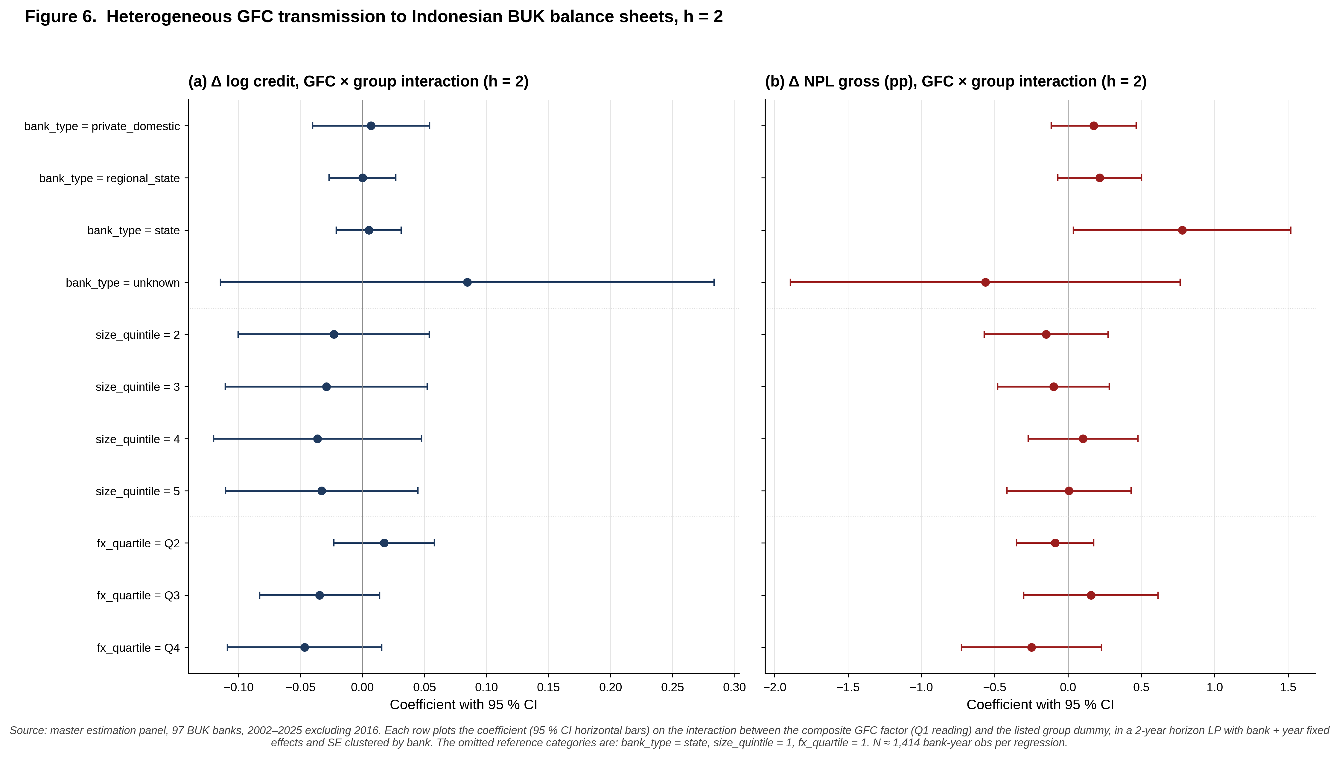
Table 3 reports the heterogeneity interactions at \(h = 2\) — the horizon at which the differential effects across bank-characteristic groups first emerge clearly while the average response is still close to zero (Table 2), allowing the cross-sectional structure to be read without contamination by the average effect. The specification follows equation (2): bank fixed effects, year fixed effects (which absorb the GFC factor main effect), and interactions of the GFC factor with ownership type, asset size quintile, and FX-exposure quartile.
6.1 Ownership dominates size
Bank ownership type is the dominant heterogeneity dimension. The size-quintile interactions are economically small and statistically insignificant across all four outcomes — neither credit, assets, NPL, nor CAR varies by within-year asset quintile in its sensitivity to the global cycle. The cross-section of Indonesian commercial banks does not respond differentially to the global cycle by size alone, a finding with direct implications for the calibration of domestic systemically-important bank (D-SIB) designations that are currently determined primarily by total assets.
Ownership, by contrast, partitions the cross-section sharply. State-owned banks (BUMN) display a significantly higher NPL response than foreign-owned banks: GFC × state = +0.778 percentage points (SE 0.378, \(p < 0.05\)). State banks bear a larger asset-quality cost during global risk-off, consistent with their concentrated lending exposure to cycle-sensitive sectors — state-owned enterprises, commodity producers, and infrastructure projects. Critically, the capital response moves in the opposite direction: GFC × state = +1.652 percentage points on CAR (SE 0.670, \(p < 0.05\)). Despite carrying more bad debt during stress, state banks see their capital ratios rise — a recapitalisation signature consistent with either direct equity support or supervisory forbearance.
A finding new to the Indonesian banking literature is that the recapitalisation signature is not confined to state ownership. Private domestic banks and regional state banks (Bank Pembangunan Daerah, BPD) show CAR interactions of comparable magnitude — +1.815 percentage points (\(p < 0.05\)) and +2.030 percentage points (\(p < 0.10\)) respectively. All three domestic ownership classes — state, regional state, and private domestic — exhibit CAR-supporting behaviour during global stress, while foreign-owned banks (the omitted reference) absorb the average compression of equation (1). This pattern argues against a state-bank-specific bailout hypothesis and in favour of a regulator-uniform mechanism: loss-recognition forbearance applied uniformly across Indonesian-resident banks plausibly transmits to capital ratios through deferred provisioning. The asset-quality signature (higher NPL) is state-bank-specific; the capital signature is domestic-bank-wide.
| Heterogeneity | Group | Δ log credit | Δ log assets | Δ NPL gross (pp) | Δ CAR (pp) |
|---|---|---|---|---|---|
| Ownership type (ref: foreign) | State (BUMN) | +0.005 (0.013) | +0.006 (0.010) | +0.778** (0.378) | +1.652** (0.670) |
| Regional state (BPD) | −0.000 (0.014) | +0.001 (0.011) | +0.216 (0.146) | +2.030* (1.198) | |
| Private domestic | +0.007 (0.024) | −0.003 (0.012) | +0.176 (0.148) | +1.815** (0.850) | |
| FX-exposure quartile (ref: Q1) | Q2 | +0.017 (0.021) | −0.001 (0.014) | −0.088 (0.134) | −1.852** (0.848) |
| Q3 | −0.035 (0.025) | −0.038** (0.018) | +0.156 (0.233) | −1.155 (1.009) | |
| Q4 | −0.047 (0.032) | −0.046** (0.019) | −0.249 (0.243) | +0.031 (2.047) | |
| Size quintile (ref: Q1, smallest) | Q2 | −0.023 (0.039) | +0.018 (0.017) | −0.149 (0.215) | −0.115 (1.468) |
| Q3 | −0.029 (0.042) | −0.009 (0.017) | −0.099 (0.194) | +1.204 (1.866) | |
| Q4 | −0.036 (0.043) | −0.015 (0.017) | +0.102 (0.191) | −0.864 (1.337) | |
| Q5 (largest) | −0.033 (0.040) | −0.006 (0.014) | +0.006 (0.216) | −0.471 (1.318) |
Notes: each cell shows the coefficient on GFC × group dummy. Year FE absorbs the main effect of GFC, so the reported coefficient is the additional response of the listed group relative to the omitted base category. Bank FE + year FE. SE clustered by bank. * p < 0.10, ** p < 0.05, *** p < 0.01.
6.2 The FX-exposure channel: assets retreat, credit holds
Banks in the upper FX-exposure quartiles deleverage materially during global risk-off, but the contraction is asymmetric across the balance sheet. The asset-growth interaction is significantly negative for Q3 (−0.038 log points, SE 0.018, \(p < 0.05\)) and Q4 (−0.046 log points, SE 0.019, \(p < 0.05\)); the credit-growth interaction carries the same sign but does not cross conventional significance (−0.035 and −0.047 log points respectively). High-FX-exposure banks shrink their total balance sheet during stress — pulling back proprietary trading positions, inter-bank exposures, and FX derivative books — while protecting their loan portfolios. The funding-shock transmission is therefore visible in the trading book before it reaches the loan book.
The asymmetric adjustment is policy-relevant. Tools targeting the lending side of the balance sheet (LTV ratios, sectoral exposure caps) bind during the contraction of the loan book, which arrives last; tools targeting the off-balance-sheet FX side (foreign-currency reserve requirements, the post-2014 corporate FX hedging rule, derivative-position caps) bind during the trading-book contraction, which arrives first. The cross-quartile sequencing observed here is consistent with the design intent of the post-2014 Indonesian FX prudential package, which targets the off-balance-sheet commitment frontier (Warjiyo 2016). Whether the binding thresholds are calibrated appropriately is a separate empirical question that the present data do not address directly.
7. Episode event-study
Table 4 reports the bank-level event-study coefficients at \(h = 2\) for each of the six pre-specified risk-off episodes (equation 3). The cross-episode pattern is heterogeneous: two episodes deliver the textbook contraction, three are statistically muted, and one delivers the polar-opposite signature.
7.1 Three regimes across the six episodes
The six episodes partition into three regimes by the sign and significance of the credit-growth coefficient. The textbook risk-off regime — GFC 2008–09 (−11.5 log points, \(p < 0.05\)) and COVID-19 2020 (−15.6 log points, \(p < 0.01\)) — produces a sharp cumulative contraction in bank-level credit over the two-year horizon. The quiet absorption regime — CNY/commodity 2015–16 (+6.5, n.s.), EM contagion 2018 (−3.3, n.s.), and Taper tantrum 2013 — registers either no significant cumulative response or a counterintuitive positive cumulative response. The inverse regime — Fed-hike cycle 2022–23 — shows positive credit growth (+9.0 log points, \(p < 0.10\)) and a negative NPL response (−129 basis points, \(p < 0.05\)). The pattern is not random across episodes: the two regimes that produce the most pronounced contraction are the two episodes that preceded the post-2016 macroprudential consolidation in Indonesia.
7.2 The textbook contractions: GFC 2008–09 and COVID 2020
The 2008 global financial crisis dummy delivers the cleanest contraction in the sample. The credit-growth coefficient is −0.115 log points (SE 0.056, \(p < 0.05\)) and the NPL response is +1.22 percentage points (SE 0.514, \(p < 0.05\)) — banks contract their loan books by roughly 11.5 per cent cumulatively over two years while simultaneously absorbing 120 basis points of new non-performing loans. The CAR response is positive but statistically noisy (+2.12 pp, SE 1.77), an early manifestation of the recapitalisation signature documented in §6.1.
The COVID-19 episode produces the sharpest credit contraction in the sample, with a coefficient of −0.156 log points (SE 0.052, \(p < 0.01\)). The NPL response is not identified for this episode because the post-2016 NPL bridge has limited overlap with the 2020 window in the parsed sample (§3.3). The COVID-19 contraction is larger in magnitude than the 2008 GFC contraction by about four log points, plausibly reflecting the more abrupt and synchronised nature of the pandemic shock relative to the post-Lehman build-up.
7.3 The intermediate episodes: muted absorption and a timing artefact
The 2015–16 Chinese renminbi devaluation and commodity bust window registers no statistically significant bank-level response (+6.5 log points on credit, n.s.; +3.7 on assets, n.s.). This is consistent with the descriptive panel of Figure 2(c), which shows that Indonesian credit growth continued through the 2015 commodity collapse with only mild deceleration. The 2018 emerging-market contagion window similarly registers no credit response (−3.3 log points, n.s.); the only marginally significant move is on asset growth (−0.040 log points, \(p < 0.10\)), indicating mild balance-sheet caution but no full contraction.
The 2013 Taper tantrum result requires careful interpretation. The coefficient on credit growth is significantly positive (+0.111 log points, \(p < 0.01\)) and on assets equally positive (+0.106 log points, \(p < 0.01\)). The sign reflects the cumulative timing of the local-projection window rather than the contemporaneous shock: the \(h = 2\) outcome compares April 2013 (the BUK snapshot during the taper) with April 2015. Basri (2017) documents that Indonesia exited the “Fragile Five” within approximately seven months of the May 2013 taper announcement through a coordinated monetary–fiscal policy response. The two-year window therefore captures both the brief contraction and the policy-mix-driven recovery; the cumulative effect dominated by the latter is positive. The Taper episode is not evidence of inverse transmission but of effective policy response within the window.
7.4 The Fed-hike 2022–23 anomaly: post-2016 macroprudential effectiveness
The most consequential episode result is the Fed-hike cycle. Between March 2022 and July 2023 the US Federal Reserve raised the policy rate by a cumulative 525 basis points — the steepest tightening cycle since the 1980s. Conventional cross-border banking theory (Bruno and Shin 2015b) predicts a sharp contraction in EM bank credit and a deterioration in asset quality. The Indonesian bank-level data show the opposite. Credit growth at \(h = 2\) is +0.090 log points (SE 0.047, \(p < 0.10\)); the NPL response is negative — −1.29 percentage points (SE 0.654, \(p < 0.05\)); the CAR response is also negative (−3.47 pp) though not statistically significant. Indonesian banks grew their loan books and improved asset quality during the largest US tightening shock of the modern era.
The contrast with 2008 is stark. The 2008 GFC episode produced −11.5 log points of credit contraction and +1.22 percentage points of NPL deterioration; the Fed-hike episode produced +9.0 log points of credit expansion and −1.29 percentage points of NPL improvement. The peak-to-trough swing between these two episodes is on the order of twenty log points of credit growth and 250 basis points of asset quality — a regime shift, not a marginal evolution.
The interpretive frame that organises this contrast is the post-2016 evolution of Indonesian macroprudential policy. By 2022 the loan-to-value ratio, the countercyclical capital buffer, the foreign-currency hedging rule for corporates, and the Komite Stabilitas Sistem Keuangan crisis-management architecture (Law No. 9/2016) were all fully operational. Section 9 develops the asymmetric-effectiveness interpretation that this episode result anchors: the post-2016 framework absorbed the downside of the Fed-hike cycle while leaving the upside of the global cycle (the slow-build credit response documented in Section 5) substantially untouched.
| Episode | Δ log credit | Δ log assets | Δ NPL gross (pp) | Δ CAR (pp) |
|---|---|---|---|---|
| GFC 2008–09 | −0.115** (0.056) | −0.052 (0.032) | +1.217** (0.514) | +2.123 (1.774) |
| Taper tantrum 2013 | +0.111*** (0.034) | +0.106*** (0.029) | — | — |
| CNY / commodity 2015–16 | +0.065 (0.067) | +0.037 (0.047) | — | — |
| EM contagion 2018 | −0.033 (0.032) | −0.040* (0.024) | — | — |
| COVID 2020 | −0.156*** (0.052) | +0.027 (0.049) | — | — |
| Fed hike 2022–23 | +0.090* (0.047) | +0.004 (0.028) | −1.290** (0.654) | −3.471 (2.282) |
Notes: coefficient on the corresponding episode dummy (1 if year overlaps the pre-specified window). NPL and CAR responses for 2013–2018 episodes are absorbed by the post-2016 NPL/CAR data bridge (§3.3). Bank fixed effects, SE clustered by bank. * p < 0.10, ** p < 0.05, *** p < 0.01.
8. Robustness
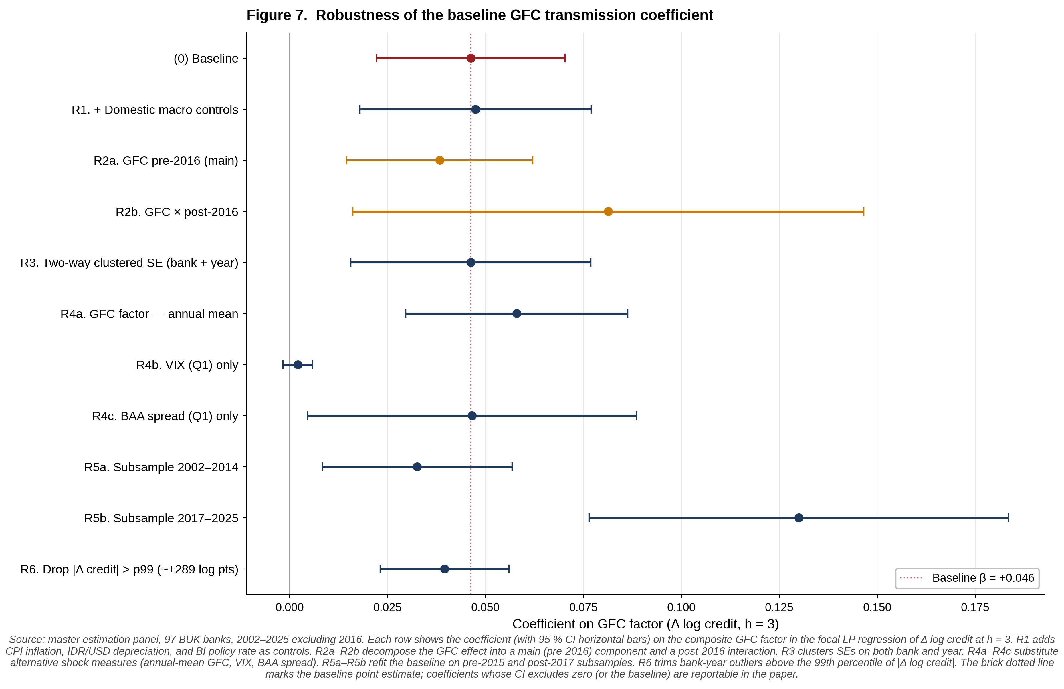
Table 5 and Figure 7 report six robustness checks for the baseline coefficient on Δ log credit at \(h = 3\) (\(\beta = +0.046\), SE 0.012). The checks fall into three categories: identification stability under alternative controls and standard-error specifications, decomposition of the composite shock to isolate the operative transmission channel, and temporal stability across the pre- and post-2016 sub-periods.
8.1 Identification stability
Three checks confirm that the baseline is not an artefact of specification choices.
R1 — Domestic macroeconomic controls. Adding contemporaneous CPI inflation, the log IDR–USD depreciation, and the Bank Indonesia policy rate leaves the GFC coefficient virtually unchanged (\(\beta = +0.047\), SE 0.015, \(p < 0.01\)). The GFC factor is not proxying for endogenous Indonesian policy response to the global cycle.
R3 — Two-way clustered standard errors. Replacing bank-clustering with two-way clustering on bank and year widens the standard error modestly (0.012 → 0.016) but the coefficient remains significant at the 1 per cent level (\(\beta = +0.046\), SE 0.016).
R6 — Outlier robustness. Dropping bank-year observations with \(|\Delta \ln \text{credit}|\) above the 99th percentile (the threshold is approximately ±289 log points and captures large M&A-driven balance-sheet jumps) yields \(\beta = +0.040\) (SE 0.008, \(p < 0.01\)). The baseline is not driven by a handful of merger-fuelled outliers.
8.2 The operative shock: credit spread, not volatility
The composite global financial cycle factor combines five US financial-market series. Substituting each component in turn identifies which component actually carries the empirical transmission.
R4a — Annual mean. Replacing the Q1 reading of the composite with its annual mean yields \(\beta = +0.058\) (SE 0.014, \(p < 0.01\)) — slightly larger than the baseline, consistent with the annual-mean signal smoothing within-year noise.
R4b — VIX alone. Substituting the standalone Q1 VIX for the composite yields \(\beta = +0.002\) (SE 0.002), statistically indistinguishable from zero. Pure equity-market volatility on its own does not transmit to Indonesian bank credit at the bank-year frequency.
R4c — BAA spread alone. Substituting the standalone Q1 Moody’s BAA–10-year corporate-credit spread yields \(\beta = +0.047\) (SE 0.021, \(p < 0.05\)) — virtually identical to the baseline composite. The credit-spread component carries essentially the full transmission of the composite factor.
The R4b/R4c contrast is substantive. The Bruno and Shin (2015b) cross-border banking model frames the global cycle through VIX-driven leverage; the Avdjiev, McCauley, and Shin (2016) extension emphasises the dollar funding channel. The Indonesian bank-level evidence here argues that for emerging-market commercial-bank credit transmission, the price of risk in corporate credit markets (Gilchrist and Zakrajšek 2012) is the operative shock — not equity-market volatility per se. This is consistent with the bank-intermediated structure of Indonesian credit: the borrowing cost in the corporate-bond market is the proximate price signal that local banks observe and respond to, while equity-market volatility is at most a leading indicator with no independent transmission once the spread is controlled for.
8.3 Temporal stability and the post-2016 intensification
The defining robustness finding is the intensification of the transmission after the 2016 consolidation of the Indonesian macroprudential framework.
R2 — Pre/post-2016 explicit interaction. Allowing the GFC effect to differ by a post-2016 dummy yields a pre-2016 coefficient of +0.038 (SE 0.012, \(p < 0.01\)) and an additional post-2016 interaction of +0.081 (SE 0.033, \(p < 0.05\)). The total post-2016 sensitivity is +0.119 log points — more than three times the pre-2016 magnitude.
R5 — Subsample re-estimation. Re-fitting the baseline equation (1) on the 2002–2014 sub-sample yields \(\beta = +0.033\) (SE 0.012, \(p < 0.01\)); re-fitting on the 2017–2025 sub-sample yields \(\beta = +0.130\) (SE 0.027, \(p < 0.01\)). The post-2017 sensitivity is approximately four times the pre-2014 magnitude. Both R2 and R5 confirm the same direction and magnitude of intensification: the transmission of the global cycle to Indonesian bank credit grew stronger, not weaker, under the consolidated post-2016 macroprudential regime.
This intensification is the central empirical fact that anchors the asymmetric-effectiveness interpretation developed in Section 9. The post-2016 framework — the countercyclical capital buffer (PBI 2015), the foreign-currency hedging rule for non-bank corporates (2014), and the KSSK crisis-management architecture (Law No. 9/2016) — was designed to contain the downside of the global cycle. The Section 7.4 result on the 2022–23 Fed-hike episode confirms this downside containment: credit expanded and asset quality improved during the steepest US tightening cycle since the 1980s. But the same framework leaves the upside of the global cycle — the slow-build credit response to accommodative phases documented in Section 5 — substantially untouched. Indeed, the upside transmission is materially stronger after 2016 than before. Section 9 develops this asymmetry as the paper’s central interpretive contribution.
| Specification | Coefficient (SE) | N obs |
|---|---|---|
| (0) Baseline | +0.046*** (0.012) | 1,757 |
| R1. + Domestic macro controls | +0.047*** (0.015) | 1,757 |
| R2a. GFC pre-2016 (main) | +0.038*** (0.012) | 1,757 |
| R2b. GFC × post-2016 (interaction) | +0.081** (0.033) | 1,757 |
| R3. Two-way clustered SE (bank + year) | +0.046*** (0.016) | 1,757 |
| R4a. GFC factor — annual mean | +0.058*** (0.014) | 1,757 |
| R4b. VIX (Q1) only | +0.002 (0.002) | 1,757 |
| R4c. BAA spread (Q1) only | +0.047** (0.021) | 1,757 |
| R5a. Subsample 2002–2014 | +0.033*** (0.012) | 1,145 |
| R5b. Subsample 2017–2025 | +0.130*** (0.027) | 521 |
| R6. Drop |Δ credit| > p99 | +0.040*** (0.008) | 1,740 |
Notes: all specifications include bank fixed effects and the baseline lagged controls (lag log assets, DPK share, credit share). * p < 0.10, ** p < 0.05, *** p < 0.01.
9. The asymmetric-macroprudential interpretation
The 2013–2025 evolution of Indonesian macroprudential policy consolidated a stack of instruments: loan-to-value ratios from 2012, the corporate foreign-currency hedging rule from 2014, the countercyclical capital buffer from 2015, and the Komite Stabilitas Sistem Keuangan crisis-management architecture from 2016 (Warjiyo 2016; Republik Indonesia 2016). A natural hypothesis is that this package should attenuate the response of Indonesian bank balance sheets to the global financial cycle. The empirical evidence assembled in Sections 5–8 supports a more specific claim: the framework is asymmetrically effective, containing the downside transmission of the cycle while leaving the upside transmission substantially untouched — and indeed amplified after 2016.
9.1 The downside is contained
Three empirical results document downside containment. First, the 2022–23 Fed-hike episode — the largest US tightening cycle since the 1980s, with the policy rate raised by a cumulative 525 basis points — produced a positive credit-growth coefficient at the bank level (+9.0 log points, \(p < 0.10\)) and a negative NPL response (−129 basis points, \(p < 0.05\)). The textbook risk-off contraction predicted by Bruno and Shin (2015b) did not materialise (§7.4). Second, all three domestic ownership classes — state, regional state, and private domestic — exhibit a CAR-supporting interaction with the GFC factor (§6.1), consistent with regulator-uniform loss-recognition forbearance applied across Indonesian-resident banks during stress. Third, banks in the upper FX-exposure quartiles deleverage their trading books before their loan books during cycle downturns (§6.2), an orderly off-balance-sheet adjustment that the post-2014 FX prudential package was designed to channel. Across the three results, the data describe a framework that prevents downside transmission from manifesting as the bank-balance-sheet stress documented in the 2008 GFC episode (−11.5 log points credit growth, +122 basis points NPL).
9.2 The upside is not contained
The same evidence does not support a symmetric containment of the upside. The pre-2016 baseline coefficient on the GFC factor for cumulative three-year credit growth is +0.038 (\(p < 0.01\), §8.3 R2). The post-2016 coefficient is +0.119 — more than three times the pre-2016 magnitude. The subsample re-estimation (§8.3 R5) confirms the direction: 2017–2025 sensitivity is +0.130 against 2002–2014 sensitivity of +0.033, an approximately four-fold intensification. Far from dampening the upside transmission, the post-2016 framework coexists with a stronger response of Indonesian bank credit to accommodative phases of the global cycle.
The mechanism is visible in the bank-level cross-section. The slow-build pattern of Section 5 — credit expansion peaking at the three-year horizon during accommodative phases — corresponds to the carry-trade dynamic described by Bruno and Shin (2015a) and Avdjiev, McCauley, and Shin (2016): cheap dollar funding flows into Indonesian banks, which intermediate it into local-currency credit. The credit expansion does not generate contemporaneous asset-quality deterioration (NPL falls by 25 basis points at \(h = 3\)), so the loss-recognition tools that anchor the post-2016 framework do not bind. Capital adequacy compresses (−80 basis points at \(h = 3\)) but not because of crystallised losses; the risk-weighted-asset denominator grows faster than the regulatory-capital numerator. This is asymmetric capital management at the bank level (§5.3), and it is asymmetric macroprudential effectiveness at the framework level: the policy stack constrains the loss side of the bank balance sheet, not the exposure side.
9.3 An asymmetry by design, not by failure
The asymmetric pattern is not a failure of the Indonesian macroprudential framework — it is a consequence of its instrument design. The loan-to-value ratio binds in the housing-credit market only when loan-to-value rises; it permits but does not require expansion. The countercyclical capital buffer raises required capital during booms but, at the post-2015 calibration, the binding rate has not exceeded zero percentage points outside short windows. The corporate FX hedging rule applies to non-bank corporates above a size threshold and does not bind on banks directly. The loss-recognition standards apply when losses crystallise; absent loss crystallisation, they do not bind. The framework is built around loss-given-default and capital adequacy tools rather than around exposure-cap tools. It contains downside transmission and is silent on upside transmission. Section 10 discusses which tool classes would close the upside gap.
The Indonesian single-country evidence converges with the cross-country panels of Cerutti, Claessens, and Laeven (2017), Akinci and Olmstead-Rumsey (2018), and Fendoglu (2017), all of which document that macroprudential tightening reduces credit growth less in expansions than capital buffers reduce credit contractions in contractions. The recent Frost, Ito, and van Stralen (2020) and Epure, Mihai, Minoiu, and Peydró (2024) updates extend the pattern to the global-cycle interaction specifically: when the VIX is low and global funding is cheap, macroprudential policies shift cycle transmission across credit categories rather than eliminate it. This paper documents the same asymmetric signature using granular bank-balance-sheet data within a single jurisdiction, over a 23-year window covering six global risk-off episodes. To the author’s knowledge, it is the first such single-country bank-level test of asymmetric macroprudential effectiveness in Indonesia.
10. Discussion and policy implications
The asymmetric-effectiveness pattern identified in Section 9 carries direct implications for the calibration and instrument design of Indonesian macroprudential policy. Four implications, grouped by policy lever, emerge from the bank-level evidence assembled here.
10.1 Closing the upside gap: exposure-cap tools
The defining gap identified by this paper is the upside transmission that the post-2016 framework leaves unconstrained. The framework relies primarily on loss-recognition and capital-adequacy instruments — LTV ratios, the countercyclical capital buffer, loss-provisioning standards — that bind only when losses crystallise or capital ratios approach regulatory minima. During accommodative phases of the global cycle, when NPL ratios fall and CAR remains comfortably above the Basel minimum (the median bank in this sample carries a CAR of 22 per cent against the 8 per cent floor; Table 1), these instruments do not bind.
Closing the upside gap requires exposure-cap tools that target the bank balance sheet directly rather than through the loss channel. Three candidate instruments are particularly relevant for the Indonesian setting. First, foreign-currency reserve requirements on bank liabilities, which raise the marginal cost of cross-border dollar funding directly and would target the carry-trade dynamic documented in Sections 5–6. Bank Indonesia already operates a Giro Wajib Minimum Valas (GWM Valas) regime, but the historical binding calibration has been low; the post-2016 intensification of credit transmission documented in §8.3 — a three-to-four-fold increase in sensitivity — suggests that the binding rate could be raised meaningfully without disrupting the underlying credit-supply function. Second, surge-cyclical calibration of the countercyclical capital buffer that uses the BAA corporate-credit-spread component identified in §8.2 R4c as the activation trigger rather than aggregate credit-to-GDP. The spread is observed continuously, leads the bank-level credit response by approximately two to three years (the slow-build pattern of §5.1), and provides operational lead time to activate the buffer. Third, exposure caps on the off-balance-sheet FX commitments of the highest-exposure banks (Q3 and Q4 in §6.2), where the deleveraging-then-loan-book sequencing already operates and a binding cap would simply formalise the orderly adjustment observed in the data.
10.2 Calibration insights from heterogeneity
The cross-sectional structure of the response identified in Section 6 has direct calibration implications. Most importantly, ownership type dominates asset size in the heterogeneity of cycle transmission: the size-quintile interactions are uniformly insignificant, while the ownership interactions partition the cross-section sharply (§6.1). Macroprudential frameworks that rely primarily on size-based systemically-important-bank designations therefore miss the relevant heterogeneity dimension. A revised D-SIB methodology that weights ownership type and FX-exposure quartile alongside total assets would target the actual cross-cycle variance.
A related implication concerns the recapitalisation signature documented across all three domestic ownership classes (§6.1). The pattern is consistent with regulator-uniform loss-recognition forbearance during stress — an effective stabilisation mechanism in the short run but one that can mask the buildup of asset-quality vulnerabilities. A forbearance budget — explicit ex-ante rules governing the size and duration of permissible deferral, with disclosure to supervisors and reversal triggers — would preserve the short-run stabilising function while limiting the accumulation of off-balance-sheet credit risk.
10.3 The credit-spread channel: implications for monitoring
The R4b/R4c decomposition in §8.2 carries a specific implication for macroprudential surveillance: the operative shock from the global cycle is the corporate-credit spread, not equity-market volatility. The VIX, the most-watched cross-border-cycle proxy in the post-Bruno-Shin literature, has no measurable independent effect on Indonesian bank credit at the bank-year frequency once the BAA spread is controlled for. The implication for Bank Indonesia’s macroprudential surveillance dashboard is that the relevant external indicator is the corporate-credit-spread component of US financial conditions — and, by extension, the Indonesian corporate-bond spread, which would carry the analogous signal for domestic credit conditions. Indicator-based monitoring frameworks built around the VIX or aggregate financial conditions indices may misread the cycle signal that matters for bank credit.
10.4 Limitations and future research
Three limitations should be noted. First, the parsed OJK panel is annual; quarterly variation in CAR and NPL is not observed within years, because the OJK public archive releases these variables only at the Q1 (April) snapshot for the entire 2002–2025 sample (§3.1, Appendix A.1). Local projections at annual frequency lose power against short-lived shocks, of which the Taper tantrum (§7.3) is the clearest example. The post-2021 transition to quarterly triwulanan releases would, with sufficient additional sample length, permit a follow-up paper at the quarterly frequency. Second, the 2016 fiscal-year gap reduces the effective sample by one year; this gap is structural in the OJK public archive and is absorbed into year fixed effects in the empirical specifications. Third, the bank ownership classification is static, derived from 2021–2024 susunan records (§3.5, Appendix A.5); pre-2021 ownership changes from foreign acquisitions, BUMN consolidations, and M&A are not captured. A robustness exercise using historical ownership records — sourced from the OJK annual reports rather than the susunan panel — would extend the cross-sectional identification.
Two extensions are particularly promising. The first is a loan-level credit-register analysis along the lines of Epure, Mihai, Minoiu, and Peydró (2024) for Romania, which would identify the borrower-side mechanism through which Indonesian banks intermediate the global cycle. The second is a structural model of the FX-exposure-cap calibration question raised in §10.1 — what binding rate on the GWM Valas would compress the cross-sectional p90 of the FX-exposure distribution into a targeted range while preserving the underlying credit-supply function. Both extensions require richer data than the present public archive provides and are flagged here as natural follow-ups.
11. Conclusion
This paper has asked how the global financial cycle transmits to Indonesian commercial bank balance sheets, using a public-data panel of all 97 Bank Umum Konvensional over 2002–2025 and a sequence of local projections of cumulative credit, asset, NPL, and CAR responses to a composite global financial cycle factor. Four results stand out. The unconditional annual correlation between the global cycle and median bank-level credit growth is weak (+0.19), but bank-level local projections recover an economically meaningful three-year credit response of +4.6 log points per one-standard-deviation shock to the cycle factor (\(p < 0.01\)). The credit response is accompanied by improving asset quality (NPL falls 25 basis points) and compressing capital ratios (CAR falls 80 basis points) at the same horizon — an asymmetric capital-management triad consistent with banks building leverage on improving fundamentals during accommodative phases of the cycle. Ownership type, not bank size, dominates the heterogeneous response; the operative shock is the BAA corporate-credit spread, not equity-market volatility; and the post-2016 sensitivity is roughly four times the pre-2014 magnitude.
The interpretive thread running through these results is asymmetric macroprudential effectiveness. The Indonesian framework consolidated by 2016 — loan-to-value ratios, the countercyclical capital buffer, the corporate FX hedging rule, and the Komite Stabilitas Sistem Keuangan crisis architecture — contains the downside transmission of the cycle, as the 2022–23 Fed-hike episode confirms (credit expanded and asset quality improved through the steepest US tightening cycle since the 1980s). The same framework does not contain the upside transmission, which has materially intensified post-2016 rather than dampened. This is not a framework failure but a consequence of instrument design: loss-recognition and capital-adequacy tools bind on losses, not on exposures. Closing the upside gap requires exposure-cap instruments — foreign-currency reserve requirements, surge-cyclical countercyclical buffer calibration triggered by the credit-spread component, and binding FX-exposure caps on the highest-exposure banks.
The Indonesian single-country bank-level evidence converges with the cross-country panels of Cerutti, Claessens, and Laeven (2017), Akinci and Olmstead-Rumsey (2018), and Fendoglu (2017). To the author’s knowledge, this paper is the first such single-country test of asymmetric macroprudential effectiveness using granular bank balance-sheet data in Indonesia, over a 23-year window covering six major global risk-off episodes. The framework architecture is mature; the calibration frontier — particularly on the exposure-cap side — remains open.
References
Akinci, Ozge, and Jane Olmstead-Rumsey. 2018. “How Effective Are Macroprudential Policies? An Empirical Investigation.” Journal of Financial Intermediation 33: 33–57.
Aldasoro, Iñaki, Stefan Avdjiev, Claudio Borio, and Piti Disyatat. 2023. “Global and Domestic Financial Cycles: Variations on a Theme.” International Journal of Central Banking 19 (5): 49–98.
Almuzara, Martín, and Víctor Sancibrián. 2024. “Micro Responses to Macro Shocks.” Federal Reserve Bank of New York Staff Reports No. 1090.
Arnabal, Luis Rodrigo, Santiago Camara, and Cecilia Dassatti. 2025. “Global Banks’ Spillovers to Emerging Markets: Macro to Micro Transmission.” Working paper, arXiv:2512.01132.
Avdjiev, Stefan, Robert N. McCauley, and Hyun Song Shin. 2016. “Breaking Free of the Triple Coincidence in International Finance.” Economic Policy 31 (87): 409–451.
Basri, M. Chatib. 2017. “India and Indonesia: Lessons Learned from the 2013 Taper Tantrum.” Bulletin of Indonesian Economic Studies 53 (2): 137–160.
Borio, Claudio, and Piti Disyatat. 2011. “Global Imbalances and the Financial Crisis: Link or No Link?” BIS Working Paper No. 346.
Bräuning, Falk, and Victoria Ivashina. 2020. “U.S. Monetary Policy and Emerging Market Credit Cycles.” Journal of Monetary Economics 112: 57–76.
Bruno, Valentina, and Hyun Song Shin. 2015a. “Cross-Border Banking and Global Liquidity.” Review of Economic Studies 82 (2): 535–564.
Bruno, Valentina, and Hyun Song Shin. 2015b. “Capital Flows and the Risk-Taking Channel of Monetary Policy.” Journal of Monetary Economics 71: 119–132.
Calvo, Guillermo A., Leonardo Leiderman, and Carmen M. Reinhart. 1993. “Capital Inflows and Real Exchange Rate Appreciation in Latin America: The Role of External Factors.” IMF Staff Papers 40 (1): 108–151.
Catalán, Mario, Alexander W. Hoffmaister, and Cicilia A. Harun. 2020. “Bank Capital and Lending: Evidence of Nonlinearity from Indonesia.” Journal of Asian Economics 68: 101199.
Cerutti, Eugenio, Stijn Claessens, and Lev Ratnovski. 2017. “Global Liquidity and Cross-Border Bank Flows.” Economic Policy 32 (89): 81–125.
Cerutti, Eugenio, Stijn Claessens, and Luc Laeven. 2017. “The Use and Effectiveness of Macroprudential Policies: New Evidence.” Journal of Financial Stability 28: 203–224.
Dąbrowski, Marek A., and Dimas Mukhlas Widiantoro. 2023. “Effectiveness and Conduct of Macroprudential Policy in Indonesia in 2003–2020: Evidence from the Structural VAR Models.” Eurasian Economic Review 13 (3): 703–731.
Epure, Mircea, Irina Mihai, Camelia Minoiu, and José-Luis Peydró. 2024. “Global Financial Cycle, Household Credit, and Macroprudential Policies.” Management Science 70 (11): 8096–8115.
Fendoglu, Salih. 2017. “Credit Cycles and Capital Flows: Effectiveness of the Macroprudential Policy Framework in Emerging Market Economies.” Journal of Banking and Finance 79: 110–128.
Forbes, Kristin J., and Francis E. Warnock. 2012. “Capital Flow Waves: Surges, Stops, Flight, and Retrenchment.” Journal of International Economics 88 (2): 235–251.
Frost, Jon, Hiro Ito, and René van Stralen. 2020. “The Effectiveness of Macroprudential Policies and Capital Controls Against Volatile Capital Inflows.” BIS Working Paper No. 867.
Gilchrist, Simon, and Egon Zakrajšek. 2012. “Credit Spreads and Business Cycle Fluctuations.” American Economic Review 102 (4): 1692–1720.
International Monetary Fund. 2024a. Indonesia: 2024 Article IV Consultation — Press Release; Staff Report; and Statement by the Executive Director for Indonesia. IMF Country Report No. 24/270. Washington, DC: IMF.
International Monetary Fund. 2024b. Indonesia: Financial Sector Assessment Program — Financial System Stability Assessment. IMF Country Report No. 24/272. Washington, DC: IMF.
International Monetary Fund. 2025a. Global Financial Stability Report, October 2025: Shifting Ground beneath the Calm. Washington, DC: IMF.
International Monetary Fund. 2025b. “Emerging Market Resilience: Good Luck or Good Policies?” World Economic Outlook Chapter 2, October.
Jordà, Òscar. 2005. “Estimation and Inference of Impulse Responses by Local Projections.” American Economic Review 95 (1): 161–182.
Jordà, Òscar, and Alan M. Taylor. 2023. “Local Projections for Applied Economics.” Annual Review of Economics 15: 607–631.
Miranda-Agrippino, Silvia, and Hélène Rey. 2020. “U.S. Monetary Policy and the Global Financial Cycle.” Review of Economic Studies 87 (6): 2754–2776.
Miranda-Agrippino, Silvia, and Hélène Rey. 2022. “The Global Financial Cycle.” In Handbook of International Economics Vol. 6, edited by Gita Gopinath, Elhanan Helpman, and Kenneth Rogoff, 1–43. Amsterdam: Elsevier.
Montiel-Olea, José Luis, and Mikkel Plagborg-Møller. 2021. “Local Projection Inference Is Simpler and More Robust Than You Think.” Econometrica 89 (4): 1789–1823.
Plagborg-Møller, Mikkel, and Christian K. Wolf. 2021. “Local Projections and VARs Estimate the Same Impulse Responses.” Econometrica 89 (2): 955–980.
Republik Indonesia. 2016. Undang-Undang Nomor 9 Tahun 2016 tentang Pencegahan dan Penanganan Krisis Sistem Keuangan (PPKSK). Jakarta: Sekretariat Negara.
Rey, Hélène. 2013. “Dilemma not Trilemma: The Global Financial Cycle and Monetary Policy Independence.” Proceedings of the Federal Reserve Bank of Kansas City Economic Policy Symposium, Jackson Hole.
Rey, Hélène. 2016. “International Channels of Transmission of Monetary Policy and the Mundellian Trilemma.” IMF Economic Review 64 (1): 6–35.
Soedarmono, Wahyoe, Iman Gunadi, Sudiro Pambudi, and Tika Nurhayati. 2021. “The Bank Lending Channel Revisited: Evidence from Indonesia.” Bank Indonesia Working Paper WP/04/2021.
Soedarmono, Wahyoe, Iman Gunadi, Fiskara Indawan, and Carla Sheila Wulandari. 2022. “The Dynamics of Foreign Capital Flows in Indonesia: Sources and Implications on Bond Market and Bank Stability.” Bank Indonesia Working Paper WP/03/2022.
Warjiyo, Perry. 2016. “Indonesia: The Macroprudential Framework and the Central Bank’s Policy Mix.” BIS Papers No. 94, 189–205.
Warjiyo, Perry, and Solikin M. Juhro. 2019. Central Bank Policy: Theory and Practice. Bingley: Emerald Publishing.
Appendix A. Data construction details
A.1 OJK CFS scraping and parsing pipeline
The bank-level data come from the Otoritas Jasa Keuangan (OJK) Commercial Bank Financial Reports system (Catatan atas Laporan Keuangan, CFS), publicly available at cfs.ojk.go.id. The full universe of Bank Umum Konvensional (BUK) report files for 2002–2025 is scraped and parsed, yielding 17,377 successfully parsed Excel files for 97 banks and 15 distinct report types. The parsed files are loaded into a SQLite database of 1.63 million financial observations, 26,096 ownership-and-board records, and a parse log of 17,389 entries. The parse success rate is 99.93 per cent.
The OJK CFS archive has three structural features that shape the analysis. First, the balance-sheet variables in Section 3.2 come from the posisi_keuangan_bulanan report type, which the OJK archive publishes as a single April snapshot per bank-year (denoted YYYY-B in the database) for the entire 2002–2025 sample. A separate quarterly variant (posisi_keuangan_triwulanan) is available from 2021 onwards but is not used here, both to maintain frequency consistency with the pre-2021 sub-sample and to align bank observation timing with the Q1 reading of the annual GFC factor. Second, OJK transitioned its reporting templates around 2015–2016, with the new format taking full effect in 2021 in the parsed sample. Third, fiscal year 2016 returns no_report for all banks and all report types in the OJK public endpoint, reflecting the format transition; the 2016 gap is treated as a structural one-year absence absorbed into year fixed effects.
A.2 Outcome variable bridging
The pre-2010 OJK reports label total assets as total aktiva and the 2010+ reports as total aset; the spliced series is continuous in level. Total credit similarly bridges kredit yang diberikan (pre-2010) and kredit (2010+). DPK is the sum of giro (demand deposits), tabungan (savings), simpanan berjangka (term deposits), and deposito; bank-to-bank deposit items are excluded by virtue of their distinct labels.
A.3 Risk variable bridging
CAR and NPL gross are constructed by bridging two reporting templates. For 2002–2015, CAR is the tersedia (achieved) ratio from kpmm_konsolidasi (Basel I → II.5 phase-in with four label variants by year, all extracted and concatenated). NPL gross is computed as the ratio (KL + D + M) / Jumlah from the consolidated credit row of kualitas_aktiva_produktif, where KL, D, and M are the substandard, doubtful, and loss categories of the OJK asset-quality classification. For 2021–2025, both CAR and NPL gross are taken directly from the rasio_keuangan report, with cross-validation against kpmm_car and the recomputed kualitas_aset series. Within-new-format concordance is high (Pearson r = 0.9995 for CAR; r = 0.9835 for NPL). Bank-quarter overlap between old and new templates does not exist in the parsed sample; the transition between the two sub-periods is therefore validated through the continuity of cross-sectional moments.
A.4 Foreign-currency exposure proxy construction
Eleven account labels are flagged as foreign-currency in nature: the explicit valuta asing rows, posisi pembelian/penjualan spot dan derivatif yang masih berjalan, posisi valas yang akan diserahkan/diterima, l/c luar negeri, and the terkait dengan nilai tukar block of the spot_derivatif report. The FX exposure ratio is defined as the sum of these items divided by total assets. Cross-validation between the April-bulanan and Q1-triwulanan extraction yields Pearson r = 0.925 (Spearman ρ = 0.975) on the overlap window. Ratios above 500 per cent of book assets — observed for a small number of foreign-bank branches with large notional contracts — are dropped as suspect.
A.5 Bank ownership classification rules
Ownership type is derived from the 2021–2024 susunan (ownership disclosure) records. For each bank, the dominant owner over the four-year window is identified and a type assigned based on a pattern match: the four major BUMN banks are hard-coded (codes 002, 008, 009, 200); regional governments are recognised by the substring “Pemerintah” in the dominant-owner field; foreign-owned banks are identified by a regular-expression match against common foreign-corporate suffixes (“Ltd”, “Pte”, “Limited”, “Corporation”, “Inc.”, “AG”, “PCL”, “S.A.”, country names, and the names of the world’s major global banking groups). Four banks lack 2021–2024 susunan records and are classified by their OJK code block. The resulting distribution is 4 state, 20 regional state, 38 private domestic, 31 foreign-owned, and 4 unknown.
A.6 GFC factor PCA construction
The composite global financial cycle factor is the first principal component (PC1) of five z-scored daily series from FRED, aggregated to quarterly means: VIXCLS (CBOE volatility index), DTWEXBGS (broad US dollar index, spliced with DTWEXM for 2002–2005), DFF (effective Fed Funds rate), DGS10 (US 10-year Treasury yield), and BAA10Y (Moody’s BAA — 10-year Treasury corporate spread). PC1 explains 48.2 per cent of the cross-indicator variance (PC2: 23.7 per cent; PC3: 20.5 per cent). The sign of PC1 is aligned so that VIX loads positively, ensuring that positive values indicate risk-off conditions, marked by elevated VIX and credit spreads alongside accommodative US policy rates (the Fed Funds rate loads −0.55 on PC1). Both the Q1 reading of the composite (which matches the April BUK snapshot timing) and the annual mean (used in robustness) are retained.
Appendix B. Descriptive tables
Tables referenced in the data section but not embedded in the main narrative are collected here for reference. Tables 1, 2, 3, 4, and 5 are embedded in the relevant sections of the main text.
Table B1 — Summary statistics of global risk-off indicators, 2002Q1–2025Q4
| Variable | Units | FRED ID | N | Mean | SD | Min | P10 | P90 | Max |
|---|---|---|---|---|---|---|---|---|---|
| VIX | Index points | VIXCLS | 96 | 19.44 | 7.5 | 10.31 | 12.78 | 28.67 | 58.6 |
| Broad USD index | Index (Mar 1973 = 100, spliced) | DTWEXBGS (spliced DTWEXM 2002–2005) | 96 | 106.49 | 12.08 | 86.81 | 91.21 | 121.69 | 131.51 |
| Fed Funds rate | % per annum | DFF | 96 | 1.75 | 1.85 | 0.06 | 0.09 | 5.03 | 5.33 |
| US 10Y Treasury yield | % per annum | DGS10 | 96 | 3.14 | 1.14 | 0.65 | 1.67 | 4.53 | 5.11 |
| BAA – 10Y spread | Percentage points | BAA10Y | 96 | 2.46 | 0.74 | 1.46 | 1.69 | 3.22 | 5.58 |
| Composite GFC factor (PC1) | z-score (sign: risk-off positive) | — (PCA, this paper) | 96 | 0 | 1.55 | -2.85 | -2.36 | 1.57 | 4.96 |
PCA variance explained: PC1 48.2%, PC2 23.7%, PC3 20.5%.
PC1 loadings (sign-aligned so VIX > 0 = tighter global conditions):
              PC1    PC2    PC3
vix         0.414  0.649  0.132
dxy        -0.208  0.215  0.892
ffr        -0.549  0.365 -0.051
us10y      -0.415  0.526 -0.411
baa_spread  0.558  0.350 -0.121
Table B2 - FX exposure summary, BUK Indonesia 2002-2025
FX exposure ratio = sum of foreign-currency off-balance-sheet commitments / total assets. All entries in percent.
Panel A - Distribution by year
| year | n_banks | mean | median | p25 | p75 | p90 |
|---|---|---|---|---|---|---|
| 2002 | 72 | 15.46 | 0.83 | 0 | 15.84 | 38.25 |
| 2003 | 70 | 17.88 | 0.69 | 0 | 5.84 | 37.68 |
| 2004 | 69 | 18.82 | 0.75 | 0 | 12.65 | 43.14 |
| 2005 | 74 | 15.92 | 0.65 | 0 | 4.52 | 40.62 |
| 2006 | 59 | 19.12 | 0.99 | 0.07 | 16.85 | 40.51 |
| 2007 | 59 | 16.78 | 1.05 | 0.08 | 16.72 | 47.35 |
| 2008 | 56 | 19.95 | 1.71 | 0.21 | 23.25 | 52.59 |
| 2009 | 57 | 14.66 | 1.55 | 0.25 | 6.88 | 47.04 |
| 2010 | 95 | 18.85 | 0.28 | 0 | 7.51 | 60.66 |
| 2011 | 96 | 21.54 | 0.47 | 0 | 12.71 | 63.85 |
| 2012 | 96 | 25.15 | 0.38 | 0 | 10.93 | 78.23 |
| 2013 | 95 | 21.47 | 0.42 | 0 | 13.46 | 87.61 |
| 2014 | 95 | 22.01 | 0.61 | 0 | 13.2 | 96.08 |
| 2015 | 95 | 19.67 | 0.21 | 0 | 11.11 | 58.3 |
| 2017 | 93 | 29.9 | 0.44 | 0 | 10.61 | 77.46 |
| 2018 | 92 | 24.44 | 0.7 | 0 | 13.79 | 72.01 |
| 2019 | 90 | 29.46 | 0.46 | 0 | 15.09 | 90.2 |
| 2020 | 88 | 30.83 | 0.94 | 0 | 19.32 | 79 |
| 2021 | 88 | 24.96 | 0.97 | 0 | 13.52 | 67.62 |
| 2022 | 85 | 21.83 | 1.07 | 0 | 14.31 | 60.32 |
| 2023 | 84 | 23.1 | 1.56 | 0 | 12.27 | 64.71 |
| 2024 | 85 | 28.32 | 1.75 | 0 | 21.18 | 80.87 |
| 2025 | 84 | 33.06 | 2.75 | 0 | 17.93 | 100.53 |
Panel B - Top 10 banks by average FX exposure ratio
| Bank code | Bank name | Ownership | n periods | Mean ratio (%) | Max ratio (%) |
|---|---|---|---|---|---|
| 057 | PT Bank BNP Paribas Indonesia | Foreign | 23 | 243.93 | 461.69 |
| 050 | Standard Chartered Bank | Foreign | 23 | 192.73 | 431.40 |
| 042 | MUFG Bank, Ltd | Foreign | 28 | 169.52 | 476.57 |
| 061 | PT Bank ANZ Indonesia | Foreign | 22 | 143.82 | 452.03 |
| 030 | American Express Bank Ltd. | Foreign | 7 | 136.23 | 213.84 |
| 048 | PT Bank Mizuho Indonesia | Foreign | 28 | 132.60 | 205.96 |
| 033 | Bank of America, N.A. | Foreign | 21 | 105.89 | 315.38 |
| 069 | Bank of China (Hong Kong) Limited | Foreign | 23 | 104.50 | 464.16 |
| 041 | The Hongkong and Shanghai Banking Corp (HSBC) | Foreign | 16 | 92.07 | 306.44 |
| 949 | PT Bank CTBC Indonesia | Foreign | 28 | 83.80 | 238.41 |
Note: All ten banks in the top FX-exposure decile are foreign-owned branches or subsidiaries of foreign banking groups, consistent with the cross-border carry-trade transmission channel discussed in §6.2.
Source: OJK Commercial Bank Quarterly/Monthly Financial Reports (CFS-BUK), 97 banks, 2002-2025.
Table B3. Bridge validation for CAR and NPL gross
Panel A. Coverage by sub-period and source format
| variable | bucket | source_format | n_obs |
|---|---|---|---|
| CAR | 2002-2010 | old_kpmm_konsolidasi | 708 |
| CAR | 2011-2020 | old_kpmm_konsolidasi | 344 |
| CAR | 2021-2025 | new_rasio_keuangan | 429 |
| NPL_gross | 2002-2010 | old_kualitas_aktiva_produktif | 860 |
| NPL_gross | 2011-2020 | old_kualitas_aktiva_produktif | 382 |
| NPL_gross | 2021-2025 | new_rasio_keuangan | 435 |
Panel B. Overlap validation (within new-format concordance)
| variable | overlap_N | pearson_r | mean_abs_dev_pp | mean_primary | mean_secondary |
|---|---|---|---|---|---|
| CAR | 429 | 0.999 | 0.056 | 35.547 | 35.503 |
| NPL_gross | 434 | 0.983 | 0.120 | 2.741 | 2.712 |
Panel C. Final unified panel summary statistics
| variable | n_bank_quarters | n_unique_banks | first_period | last_period | mean_pct | median_pct | p10_pct | p90_pct |
|---|---|---|---|---|---|---|---|---|
| CAR | 1481 | 95 | 2002-Q1 | 2025-Q1 | 28.391 | 22.248 | 13.710 | 45.900 |
| NPL_gross | 1677 | 97 | 2002-Q1 | 2025-Q1 | 3.675 | 2.351 | 0.324 | 6.700 |
Notes. source_format indicates the underlying OJK report from which the observation was extracted. The ‘primary’ series in Panel B is rasio_keuangan (the published headline ratio); the ‘secondary’ series is independently recomputed from kpmm_car for CAR and from kualitas_aset for NPL gross. There is no direct OLD/NEW bank-quarter overlap in the source database because the OLD KPMM and asset quality templates were discontinued after 2014-Q1 and the new templates start at 2021-Q1; the within-new-format validation reported here is the tightest concordance check the data permit, and is interpreted as a lower bound on the splice quality.
Table B4 — Outcome variables, summary statistics by sub-period
| Variable | Period | N | Mean | SD | p10 | Median | p90 |
|---|---|---|---|---|---|---|---|
| Total assets (IDR bn) | 2002–2015 | 1349 | 25570.2 | 69876 | 421.45 | 4520.04 | 54635.7 |
| Total credit (IDR bn) | 2002–2015 | 1347 | 14842 | 43202.3 | 210.33 | 2409.47 | 32061.9 |
| Total DPK (IDR bn) | 2002–2015 | 1347 | 19216.4 | 53955.8 | 263.1 | 3283.24 | 39173.8 |
| Credit share of assets (%) | 2002–2015 | 1347 | 55.84 | 19.47 | 30.24 | 58.39 | 75.41 |
| Asset growth, YoY (%) | 2002–2015 | 1250 | 17.43 | 22.59 | -4.32 | 15.72 | 41.56 |
| Credit growth, YoY (%) | 2002–2015 | 1243 | 21.12 | 27.36 | -1.57 | 20.13 | 46.82 |
| DPK growth, YoY (%) | 2002–2015 | 1244 | 16.53 | 25.69 | -8.21 | 15.23 | 43.3 |
| Total assets (IDR bn) | 2017–2025 | 803 | 101237 | 250388 | 6159.93 | 24112.5 | 185225 |
| Total credit (IDR bn) | 2017–2025 | 803 | 61918.4 | 161794 | 3016.58 | 13165 | 115905 |
| Total DPK (IDR bn) | 2017–2025 | 803 | 72342.7 | 188422 | 3915.29 | 16668.8 | 124588 |
| Credit share of assets (%) | 2017–2025 | 803 | 57.41 | 14.26 | 39.02 | 60.28 | 72.98 |
| Asset growth, YoY (%) | 2017–2025 | 801 | 10.74 | 22.15 | -6.37 | 7.53 | 28.82 |
| Credit growth, YoY (%) | 2017–2025 | 798 | 9.65 | 25.43 | -11.7 | 7.36 | 30.14 |
| DPK growth, YoY (%) | 2017–2025 | 795 | 9.31 | 24.92 | -11.7 | 7.22 | 29.31 |
| Total assets (IDR bn) | 2002–2025 | 2152 | 53804.6 | 166659 | 704.28 | 11061.2 | 117380 |
| Total credit (IDR bn) | 2002–2025 | 2150 | 32424.5 | 107038 | 346.22 | 5892.84 | 65737.5 |
| Total DPK (IDR bn) | 2002–2025 | 2150 | 39058.5 | 125434 | 446.9 | 7537.91 | 80150.5 |
| Credit share of assets (%) | 2002–2025 | 2150 | 56.43 | 17.72 | 32.44 | 59.06 | 74.23 |
| Asset growth, YoY (%) | 2002–2025 | 2051 | 14.82 | 22.65 | -5.42 | 12.16 | 38.85 |
| Credit growth, YoY (%) | 2002–2025 | 2041 | 16.64 | 27.2 | -6.61 | 13.95 | 42.64 |
| DPK growth, YoY (%) | 2002–2025 | 2039 | 13.72 | 25.63 | -9 | 11.71 | 38.77 |
Notes: All variables are annual snapshots (April / Q2). IDR billions = IDR millions / 1,000. Year-on-year growth is the first difference of log levels; |growth| > 200 % is dropped as a likely M&A artefact. 2016 is absent from the source database (gap in BUK April-2016 snapshots).
Table B5 — Master estimation panel, full-sample descriptives
| Variable | N | Mean | SD | p10 | Median | p90 |
|---|---|---|---|---|---|---|
| Total assets (IDR trillion) | 2152 | 53.805 | 166.659 | 0.704 | 11.061 | 117.38 |
| Total credit (IDR trillion) | 2150 | 32.424 | 107.038 | 0.346 | 5.893 | 65.737 |
| Total DPK (IDR trillion) | 2150 | 39.058 | 125.434 | 0.447 | 7.538 | 80.151 |
| Credit / assets | 2150 | 0.564 | 0.177 | 0.324 | 0.591 | 0.742 |
| DPK / assets | 2150 | 0.713 | 0.17 | 0.469 | 0.762 | 0.865 |
| Asset growth YoY (∆ln) | 2051 | 0.148 | 0.227 | -0.054 | 0.122 | 0.388 |
| Credit growth YoY (∆ln) | 2041 | 0.166 | 0.272 | -0.066 | 0.14 | 0.426 |
| DPK growth YoY (∆ln) | 2039 | 0.137 | 0.256 | -0.09 | 0.117 | 0.388 |
| CAR (%) | 1481 | 28.391 | 22.196 | 13.71 | 22.248 | 45.9 |
| NPL gross (%) | 1677 | 3.675 | 6.541 | 0.324 | 2.351 | 6.7 |
| FX exposure ratio | 1879 | 0.245 | 0.597 | 0 | 0.008 | 0.741 |
| GFC factor (annual) | 2152 | -0.016 | 1.446 | -2.064 | 0.143 | 1.746 |
| GFC factor (Q1) | 2152 | 0.001 | 1.585 | -2.358 | 0.509 | 1.31 |
Sample: bank-year, 2002–2025 excluding 2016. Total bank-year observations = 2,152. Distinct banks = 97.